what travel cost method

location of the visitor¡¦s home ¡¦ how far they traveled to the site
how many times they visited the site in the past year or season
the length of the trip
the amount of time spent at the site
travel expenses
the person¡¦s income or other information on the value of their time
other socioeconomic characteristics of the visitor
other locations visited during the same trip, and amount of time spent at each
other reasons for the trip (is the trip only to visit the site, or for several purposes)
fishing success at the site (how many fish caught on each trip)
perceptions of environmental quality or quality of fishing at the site
substitute sites that the person might visit instead of this site
The value of improvements in water quality was only shown to increase the value of current beach use. However, improved water quality can also be expected to increase overall beach use.
Estimates ignore visitors from outside the Baltimore-Washington statistical metropolitan sampling area.
The population and incomes in origin zones near the Chesapeake Bay beach areas are increasing, which is likely to increase visitor-days and thus total willingness to pay.
changes in access costs for a recreational site
elimination of an existing recreational site
addition of a new recreational site
changes in environmental quality at a recreational site
number of visits from each origin zone (usually defined by zipcode)
demographic information about people from each zone
round-trip mileage from each zone
travel costs per mile
the value of time spent traveling, or the opportunity cost of travel time
exact distance that each individual traveled to the site
exact travel expenses
substitute sites that the person might visit instead of this site, and the travel distance to each
quality of the recreational experience at the site, and at other similar sites (e.g., fishing success)
perceptions of environmental quality at the site
characteristics of the site and other, substitute, sites
The travel cost method closely mimics the more conventional empirical techniques used by economists to estimate economic values based on market prices.
The method is based on actual behavior¡¦what people actually do¡¦rather than stated willingness to pay¡¦what people say they would do in a hypothetical situation.
The method is relatively inexpensive to apply.
On-site surveys provide opportunities for large sample sizes, as visitors tend to be interested in participating.
The results are relatively easy to interpret and explain.
The travel cost method assumes that people perceive and respond to changes in travel costs the same way that they would respond to changes in admission price.
The most simple models assume that individuals take a trip for a single purpose ¡¦ to visit a specific recreational site. Thus, if a trip has more than one purpose, the value of the site may be overestimated. It can be difficult to apportion the travel costs among the various purposes.
Defining and measuring the opportunity cost of time, or the value of time spent traveling, can be problematic. Because the time spent traveling could have been used in other ways, it has an "opportunity cost." This should be added to the travel cost, or the value of the site will be underestimated. However, there is no strong consensus on the appropriate measure¡¦the person¡¦s wage rate, or some fraction of the wage rate¡¦and the value chosen can have a large effect on benefit estimates. In addition, if people enjoy the travel itself, then travel time becomes a benefit, not a cost, and the value of the site will be overestimated.
The availability of substitute sites will affect values. For example, if two people travel the same distance, they are assumed to have the same value. However, if one person has several substitutes available but travels to this site because it is preferred, this person¡¦s value is actually higher. Some of the more complicated models account for the availability of substitutes.
Those who value certain sites may choose to live nearby. If this is the case, they will have low travel costs, but high values for the site that are not captured by the method.
Interviewing visitors on site can introduce sampling biases to the analysis.
Measuring recreational quality, and relating recreational quality to environmental quality can be difficult.
Standard travel cost approaches provides information about current conditions, but not about gains or losses from anticipated changes in resource conditions.
In order to estimate the demand function, there needs to be enough difference between distances traveled to affect travel costs and for differences in travel costs to affect the number of trips made. Thus, it is not well suited for sites near major population centers where many visitations may be from "origin zones" that are quite close to one another.
The travel cost method is limited in its scope of application because it requires user participation. It cannot be used to assign values to on-site environmental features and functions that users of the site do not find valuable. It cannot be used to value off-site values supported by the site. Most importantly, it cannot be used to measure nonuse values. Thus, sites that have unique qualities that are valued by non-users will be undervalued.
As in all statistical methods, certain statistical problems can affect the results. These include choice of the functional form used to estimate the demand curve, choice of the estimating method, and choice of variables included in the model.
GolfSW.com - Golf Southwest tips and reviews.
VivEcuador.com - Ecuador travel information.
TheChicagoTraveler.com - Explore Chicago.
FarmingtonValleyVisit.com - Discover Connecticut's Farmington Valley.

View source
View history
Community portal
Recent changes
Random page
Featured content
What links here
Related changes
Special pages
Printable version
Permanent link
Page information
Browse properties

Travel cost method

This article deals with the Travel Cost Method, which is often used in evaluating the economic value of recreational sites. This is particularly important in the coastal zone because of the level of use and the potential values that can be attached to the natural coastal and marine environment.

The Travel Cost Method (TCM) is one of the most frequently used approaches to estimating the use values of recreational sites. The TCM was initially suggested by Hotelling [1] and subsequently developed by Clawson [2] in order to estimate the benefits from recreation at natural sites. The method is based on the premise that the recreational benefits at a specific site can be derived from the demand function that relates observed users’ behaviour (i.e., the number of trips to the site) to the cost of a visit. One of the most important issues in the TCM is the choice of the costs to be taken into account. The literature usually suggests considering direct variable costs and the opportunity cost of time spent travelling to and at the site. The classical model derived from the economic theory of consumer behaviour postulates that a consumer’s choice is based on all the sacrifices made to obtain the benefits generated by a good or service. If the price ( [math]p[/math] ) is the only sacrifice made by a consumer, the demand function for a good with no substitutes is [math]x=f(p)[/math] , given income and preferences. However, the consumer often incurs other costs ( [math]c[/math] ) in addition to the out-of-pocket price, such as travel expenses, and loss of time and stress from congestion. In this case, the demand function is expressed as [math]x = f(p, c)[/math] . In other words, the price is an imperfect measure of the full cost incurred by the purchaser. Under these conditions, the utility maximising consumer’s behaviour should be reformulated in order to take such costs into account. Given two goods or services [math]x_1, x_2[/math] , their prices [math]p_1, p_2[/math] , the access costs [math]c_1, c_2[/math] and income [math]R[/math] , the utility maximising choice of the consumer is:

[math]max \, U = u(x_1,x_2) \quad subject \, to \quad (p_1+c_1)x_1+(p_2+c_2)x_2=R . \qquad (1)[/math]

Now, let [math]x_1[/math] denote the aggregate of priced goods and services, [math]x_2[/math] the number of annual visits to a recreational site, and assume for the sake of simplicity that the cost of access to the market goods is negligible ( [math]c_1 \approx 0[/math] ) and that the recreational site is free ( [math]p_2=0[/math] ). Under these assumptions, equation (1) can be written as:

[math]max \, U = u(x_1,x_2) \quad subject \, to \quad p_1x_1+c_2x_2=R . \qquad (2)[/math]

Under these conditions, the utility maximising behaviour of the consumer depends on:

The TCM is based on the assumption that changes in the costs of access to the recreational site [math]c_2[/math] have the same effect as a change in price: the number of visits to a site decreases as the cost per visit increases. Under this assumption, the demand function for visits to the recreational site is [math]x_2=f(c_2)[/math] and can be estimated using the number of annual visits as long as it is possible to observe different costs per visit. The basic TCM model is completed by the weak complementarity assumption, which states that trips are a non-decreasing function of the quality of the site, and that the individual forgoes trips to the recreational site when the quality is the lowest possible [3] , [4] . There are two basic approaches to the TCM: the Zonal approach (ZTCM) and the Individual approach (ITCM). The two approaches share the same theoretical premises, but differ from the operational point of view. The original ZTCM takes into account the visitation rate of users coming from different zones with increasing travel costs. By contrast, ITCM, developed by Brown and Nawas [5] and Gum and Martin [6] , estimates the consumer surplus by analysing the individual visitors’ behaviour and the cost sustained for the recreational activity. These are used to estimate the relationship between the number of individual visits in a given time period, usually a year, the cost per visit and other relevant socio-economic variables. The ITCM approach can be considered a refinement or a generalisation of ZTCM [7] .

[math]x_2 = g(c_2) . \qquad (3)[/math]

The demand function can also be estimated for non-homogeneous sub-samples introducing among the independent variables income and socio-economic variables representing individual characteristics [8] . Therefore, if an individual incurs [math]c_2^e[/math] per visit, he chooses to do [math]x_2^e[/math] visits a year, while if the cost per visit increases to [math]c_2^p[/math] the number of visits will decrease to [math]x_2^p[/math] . The cost [math]cp[/math] is the choke price, that is the cost per visit that results in zero visits. The annual user surplus (the use value of the recreational site) is easily obtained by integrating the demand function from zero to the current number of annual visits, and subtracting the total expenditures on visits.

↑ Hotelling, H. (1949), Letter, In: An Economic Study of the Monetary Evaluation of Recreation in the National Parks , Washington, DC: National Park Service.
↑ Clawson, M. (1959), Method for Measuring the Demand for, and Value of, Outdoor Recreation . Resources for the Future, 10, Washington, DC.
↑ Freeman, A.M. III. (1993). The Measurement of Environmental and Resource Values: Theory and Method , Washington, DC: Resources for the Future.
↑ Herriges, J.A., C. Kling and D.J. Phaneuf (2004), 'What’s the Use? Welfare Estimates from Revealed Preference Models when Weak Complementarity Does Not Hold', Journal of Environmental Economics and Management , 47 (1), pp. 53-68.
↑ Brown, W.G. and F. Nawas (1973), 'Impact of Aggregation on the Estimation of Outdoor Recreation Demand Functions', American Journal of Agricultural Economics , 55, 246-249.
↑ Gum, R.L. and W.E.Martin (1974), 'Problems and Solutions in Estimating the Demand for and Value of Rural Outdoor Recreation', American Journal of Agricultural Economics , 56, 558-566.
↑ Ward, F.A. and D. Beal (2000), Valuing Nature with Travel Cost Method: A Manual , Northampton: Edward Elgar.
↑ Hanley, N. and C.L. Spash (1993), Cost Benefit Analysis and the Environment , Aldershot, UK: Edward Elgar.
Definitions
Articles by Paolo Rosato
Integrated coastal zone management
Evaluation and assessment in coastal management
This page was last edited on 3 March 2022, at 21:18.
Privacy policy
About Coastal Wiki
Disclaimers

Environmental Justice Organisations, Liabilities and Trade

Mapping environmental justice.

Nuclear Energy
Oil and Gas and Climate Justice
Biomass and Land Conflicts
Mining and Ship Breaking
Environmental Health and Risk Assessment
Liabilities and Valuation
Law and Institutions
Consumption, Ecologically Unequal Exchange and Ecological Debt

Travel-cost method

The travel-cost method (TCM) is used for calculating economic values of environmental goods. Unlike the contingent valuation method, TCM can only estimate use value of an environmental good or service. It is mainly applied for determining economic values of sites that are used for recreation, such as national parks. For example, TCM can estimate part of economic benefits of coral reefs, beaches or wetlands stemming from their use for recreational activities (diving and snorkelling/swimming and sunbathing/bird watching). It can also serve for evaluating how an increased entrance fee a nature park would affect the number of visitors and total park revenues from the fee. However, it cannot estimate benefits of providing habitat for endemic species.

TCM is based on the assumption that travel costs represent the price of access to a recreational site. Peoples’ willingness to pay for visiting a site is thus estimated based on the number of trips that they make at different travel costs. This is called a revealed preference technique, because it ‘reveals’ willingness to pay based on consumption behaviour of visitors.

The information is collected by conducting a survey among the visitors of a site being valued. The survey should include questions on the number of visits made to the site over some period (usually during the last 12 months), distance travelled from visitor’s home to the site, mode of travel (car, plane, bus, train, etc.), time spent travelling to the site, respondents’ income, and other socio-economic characteristics (gender, age, degree of education, etc). The researcher uses the information on distance and mode of travel to calculate travel costs. Alternatively, visitors can be asked directly in a survey to state their travel costs, although this information tends to be somewhat less reliable. Time spent travelling is considered as part of the travel costs, because this time has an opportunity cost. It could have been used for doing other activities (e.g. working, spending time with friends or enjoying a hobby). The value of time is determined based on the income of each respondent. Time spent at the site is for the same reason also considered as part of travel costs. For example, if respondents visit three different sites in 10 days and spend only 1 day at the site being valued, then only fraction of their travel costs should be assigned to this site (e.g. 1/10). Depending on the fraction used, the final benefit estimates can differ considerably.

Two approaches of TCM are distinguished – individual and zonal. Individual TCM calculates travel costs separately for each individual and requires a more detailed survey of visitors. In zonal TCM, the area surrounding the site is divided into zones, which can be either concentric circles or administrative districts. In this case, the number of visits from each zone is counted. This information is sometimes available (e.g. from the site management), which makes data collection from the visitors simpler and less expensive.

The relationship between travel costs and number of trips (the higher the travel costs, the fewer trips visitors will take) shows us the demand function for the average visitor to the site, from which one can derive the average visitor’s willingness to pay. This average value is then multiplied by the total relevant population in order to estimate the total economic value of a recreational resource.

TCM is based on the behaviour of people who actually use an environmental good and therefore cannot measure non-use values. This method is thus inappropriate for sites with unique characteristics which have a large non-use economic value component (because many people would be willing to pay for its preservation just to know that it exists, although they do not plan to visit the site in the future).

The travel-cost method might also be combined with contingent valuation to estimate an economic value of a change (either enhancement or deterioration) in environmental quality of the NP by asking the same tourists how many trips they would make in the case of a certain quality change. This information could help in estimating the effects that a particular policy causing an environmental quality change would have on the number of visitors and on the economic use value of the NP.

For further reading:

Ward, F.A., Beal, D. (2000) Valuing nature with travel cost models. A manual. Edward Elgar, Cheltenham.

Ecosystem valuation [ www.ecosystemvaluation.org/travel_costs.htm ]

This glossary entry is based on a contribution by Ivana Logar

EJOLT glossary editors: Hali Healy, Sylvia Lorek and Beatriz Rodríguez-Labajos

One comment

I quite like reading a post that will make people think. Also, thanks for allowing me to comment!

Browse by Theme

Browse by type.

Presentations
Press Releases
Scientific Papers

Online course

Online course on ecological economics: http://www.ejolt.org/2013/10/online-course-ecological-economics-and-activism/

Academia.edu no longer supports Internet Explorer.

To browse Academia.edu and the wider internet faster and more securely, please take a few seconds to upgrade your browser .

Enter the email address you signed up with and we'll email you a reset link.

We're Hiring!
Help Center

Environmental Valuation: The Travel Cost Method

Related Papers

isabel mendes

Working Papers

Journal of Leisure Research

John Loomis

Mahidi Hasan kawsar , Muha Abdullah Al Pavel , Md Abdullah Al Mamun

Estimation of recreational benefits is an important tool for both biodiversity conservation and ecotourism development in national parks and sanctuaries. The design of this work is to estimate the recreational value and to establish functional relationship between travel cost and visitation of Lawachara National Park (LNP) in Bangladesh. This study employed zonal approach of the travel cost method. The work is grounded on a sample of 422 visitors of the LNP. Results showed that the total value of environmental assets of the LNP is 55,694,173 Taka/Year. Moreover, our suggestion based on visitors' willingness to pay is that the park entrance fee of 25 Tk per person should be introduced that could generate revenue approximate 2.3 million Taka/ year, beneficial for the park management and conservation of biodiversity.

International Journal of Academic Research in Business and Social Sciences

Kamarul Ismail

Journal of Agricultural and Applied Economics

Clement Tisdell

Discusses the implications of the economic valuation of natural resources used for tourism and relates this valuation to the concept of total economic valuation. It demonstrates how applications of the concept of total economic valuation can be supportive of the conservation of natural resources used for tourism. Techniques for valuing tourism’s natural resources are then outlined and critically evaluated. Consideration is given to travel cost methods, contingent valuation methods, and hedonic pricing approaches before concentrating on current developments of valuation techniques, such as choice modelling. The general limitations of existing methods are considered and it is argued that more attention should be given to developing guidelines that will identify ‘optimally imperfect methods’. An overall assessment concludes this article.

Journal of environmental management

John Bergstrom

In this study we estimate selected visitors' demand and value for recreational trips to settings such as developed vs. undeveloped sites in U.S. national forests in the Southern United States using the travel cost method. The setting-based approach allows for valuation of multi-activity trips to particular settings. The results from an adjusted Poisson lognormal estimator corrected for truncation and endogenous stratification reveal that economic value per trip estimates are higher for wilderness compared to day-use developed settings, overnight-use developed settings, and general forest areas. Estimates of these economic values are important to resource managers because their management decisions and actions typically control recreational settings. For example, managers control developed campground capacity in a national forest, but typically not the number of campers below the capacity constraint and the number and types of activities visitors engage in during a multi-activity...

tesfaye etensa

Recreation is a human activity, which increases visitor’s wellbeing. Following an increase in population, income and mobility the demand for recreation has been increasing in many developing countries. Hence, valuation of environmental resources enables economists to integrate environmental values into economic decision-making processes.Putting a precise and acceptable value on recreation would be valuable in resource management and need to place values that reflect the true social costs and benefits. Thus, this book presents the economic valuation of recreational benefits of Wonchi Crater Lake. In this book, recreational benefits, demand function, price elasticity of demand, the optimum entrance fee, welfare implications associated with the site and perception of the visitors are evaluated. The analysis should assist any country who endowed by environmental and natural resources and who interest to grasp the concept economic valuation of recreational benefits, and should be used fo...

Tourism Management

Choong-ki Lee

The Individual Travel Cost Method with Consumer-Specific Values of Travel Time Savings

Open access
Published: 24 June 2019
Volume 74 , pages 961–984, ( 2019 )

Cite this article

You have full access to this open access article

Mikołaj Czajkowski ORCID: orcid.org/0000-0001-5118-2308 1 ,
Marek Giergiczny 1 ,
Jakub Kronenberg 2 &
Jeffrey Englin 3

11k Accesses

27 Citations

Explore all metrics

The treatment of the opportunity cost of travel time in travel cost models has been an area of research interest for many decades. Our analysis develops a methodology to combine the travel distance and travel time data with respondent-specific estimates of the value of travel time savings (VTTS). The individual VTTS are elicited with the use of discrete choice stated preference methods. The travel time valuation procedure is integrated into the travel cost valuation exercise to create a two-equation structural model of site valuation. Since the travel time equation of the structural model incorporates individual preference heterogeneity, the full structure model provides a travel cost site demand model based upon individualized values of time. The methodology is illustrated in a study of recreational birdwatching, more specifically, visits to a ‘stork village’ in Poland. We show that the usual practice of basing respondents’ VTTS on 1/3 of their wage rate is largely unfounded and propose alternatives—including a separate component of the travel cost survey aimed at valuation of respondents’ VTTS or, as a second best, asking if they wish if their journey was shorter and for those who do—use full hourly wage as an indicator of their VTTS.

Impact of tourism development upon environmental sustainability: a suggested framework for sustainable ecotourism

The Relationship of Historical Redlining with Present-Day Neighborhood Environmental and Health Outcomes: A Scoping Review and Conceptual Model

How commuting affects subjective wellbeing

Avoid common mistakes on your manuscript.

1 Introduction

This analysis proposes a structural model of the travel cost demand approach (TCM) that includes two components. One component is used to estimate the value of travel time for each individual in the sample. The second component incorporates that value of travel time into the travel cost variable that is used in the estimation of the site demand. While the travel cost demand curve is estimated using the widely applied count methodology, the travel time component of the model is based on a discrete choice stated preference method. Our approach avoids arbitrary assumptions about an individual’s value of time in an appealing way. It also allows quite intricate valuations since the stated preference portion of the model can accommodate a wide range of travel modes, time constraints, family situations and other considerations that can affect the value of one’s time when traveling for recreation.

The individual level approach to valuing travel time utilized in this analysis is made possible by relatively recent advances in modeling preference heterogeneity in stated preference studies. The advances allow the derivation of posterior estimates of each individual’s taste parameters . We argue that utilizing individual-specific values of travel time savings, based on respondents’ stated preferences, provides a feasible method for empirically incorporating the value of travel time into travel cost demand studies. Through an empirical illustration we show that the proposed approach is tractable. All it requires is the inclusion of only a few discrete choice experiment (DCE) questions in a TCM survey and a proper econometric treatment.

Our results show that using arbitrary assumptions concerning individuals’ value of travel time savings (VTTS) equal to a given share of their wage rate (e.g., 1/3) are largely unfounded. First of all, nearly half of respondents say they do not wish their journey to the site was shorter, indicating positive utility of leisure travel. Those who wished to shorten the journey were willing to pay amounts which appear only mildly correlated with their estimated wage rates. Overall, the average consumer surplus per trip calculated from the model with individual-specific VTTS were the closest to the model which used respondents’ full wage rate included for respondents who said they wish their journey was shorter (and zero for others). We suggest using this approach as the second best, in the case eliciting individual specific VTTS was not possible.

1.1 Economics of Time: What Do We Know

In 1965 Becker postulated that “time can be converted into money”. The basic idea is that people choose how much labor to supply, given a constraint that total time available is divided among work, leisure, and travel. At its bare bones, this model implies that travel time is valued at the after-tax wage rate. This is because the Becker model assumes that time can be transferred freely between work and leisure, so any marginal savings in travel time can be used to increase labor income. This model has been expanded in many directions. A common starting point is DeSerpa ( 1971 ). This model assumes that utility is affected by commodity bundles $X = (X_{1} , \ldots ,X_{n} ,T_{1} , \ldots ,T_{n} )$ where $X_{i}$ denotes some quantity of the i -th good, while $T_{i}$ denotes the amount of time allocated to the i -th good. These goods can include both travel to a recreational site and time onsite. $T_{w}$ denotes time spent at work (which may increase or decrease utility). Each activity has a minimum time requirement $\bar{T}$ (hence constraint $T_{i} \ge \bar{T}$ ). There is also an overall time constraint $T_{w} + \sum {T_{i} } \le T^{0}$ . The budget constraint is $P_{i} X_{i} \le Y + wT_{w}$ , where $Y$ is unearned income. As a result, the problem can be stated as:

This problem can be solved by formulating a Lagrangian function, in which each constraint is associated with a Lagrange multiplier indicating how tight it is (i.e., the rate at which utility could be increased by relaxing it a little). Let $\lambda$ , $\mu$ , and $\kappa$ be the Lagrangian multipliers for the budget constraint, the overall time constraint, and the activity-specific time constraints, respectively. The solution to the optimization problem yields:

Equation ( 2 ) states that value of time as a personal resource (or simply value of leisure) equals wage rate plus the value of utility from work. If $T_{i}$ in Eq. ( 3 ) is not restricted to its minimum then by the virtue of complementary slackness condition its multiplier would be zero. Which in turn implies that VTTS = 0 and that $\frac{{\partial U/\partial T_{i} }}{\lambda } = w + \frac{{\partial U/\partial T_{w} }}{\lambda }$ , that is, the value of marginal utility from the activity $i$ would be equal to value of leisure. In other words, if a person spends on an activity more time than the minimum required (the constraint $\sum\nolimits_{i = 1}^{n} {\kappa_{i} } (T_{i} - \bar{T}) \ge 0$ is not binding), such activity would be what DeSerpa ( 1971 ) calls a pure leisure good and its value equals to the value of time as a resource. On the other hand, if $\sum\nolimits_{i = 1}^{n} {\kappa_{i} } (T_{i} - \bar{T}) = 0$ then ${{\kappa_{i} } \mathord{\left/ {\vphantom {{\kappa_{i} } \lambda }} \right. \kern-0pt} \lambda }$ can be interpreted as value of time saved (VTTS) in the activity $i$ .

Most work in the transportation field assumes traveling is a means to an end and travel time is a disutility to be minimized. However, in the recent years new concepts emerged, including the so-called positive utility of travel, which suggests that travel can provide benefits and may be motivated by factors beyond reaching activity destinations (see, e.g., Mokhtarian and Salomon 2001 ; Mokhtarian 2005 ). Positive utility of travel implies that $\partial U/\partial T_{i}$ is positive. In the extreme case, if positive utility of time offsets $w + \frac{{\partial U/\partial T_{w} }}{\lambda }$ then VTTS would be zero. However, note that VTTS = 0 does not mean that the value of time is zero.

Time is scarce and the time spent on traveling to the site as well as the time spent on the site is time that could have been devoted to other activities. The value of those lost opportunities is the time cost of the trip. It is important to distinguish between VTTS and the value of time in terms of lost opportunities. If the main goal of the analysis was to estimate benefits from a new road or any other public investment that would result in time savings then the analysis should focus on monetizing benefits from time saved. However, if the goal is to estimate consumer surplus from visiting a given site then the analysis should focus on estimating the alternative cost of time. Unfortunately, in the cases when $\frac{{\partial U/\partial T_{i} }}{\lambda } > 0$ , VTTS will underestimate the true value of time and the more similar the value of travel is to the value of time on-site, the larger the discrepancy between VTTS and the value of time in terms of lost opportunities will be.

1.2 Valuing the Opportunity Cost of Travel Time in Recreation Demand Models: Previous Research

The incorporation of the value of travel time in the TCM studies has been a source of concern since the earliest applications of this method (e.g., Clawson and Knetsch 1966 ; Johnson 1966 ). Researchers disagreed not only about how much the travel time is worth but also whether it should be included it in the model at all. Cesario ( 1976 ) provided an early cogent discussion of the incorporation of the value of time into travel cost models. Despite the decades of research into the value of time, Randall’s ( 1994 ) observation that “the cost of travel time remains an empirical mystery” remains valid and estimating the value of travel time (or, in most cases, rather the opportunity cost of time) remains a frequently discussed problem in the literature on TCM (e.g., Fletcher et al. 1990 ; Garrod and Willis 1999 ; Hanley and Barbier 2009 ).

Early on McConnell ( 1975 ) stressed the need to estimate the value of time before incorporating it in the demand function. However, uncovering the rate of substitution between money and time was long considered empirically intractable (as these trade-offs are endogenous and unobservable), even if conceptually possible. Cesario’s ( 1976 ) suggestion that commuter’s travel time values of 25–50% of an individual’s wage rate was widely adopted. Using a fraction of wage rate has remained probably the most common approach, with the compromise value of 33% being the most broadly accepted level (Hellerstein and Mendelsohn 1993 ; Englin and Cameron 1996 ; Garrod and Willis 1999 ; Gürlük and Rehber 2008 ; Egan et al. 2009 ; Huhtala and Lankia 2012 ). Critics of the wage-based approach note that it makes little sense for those without reported wages, the method would suggest their marginal utility of time is zero. That is clearly not the case (Feather and Shaw 1999 ; Parsons 2003 ). Footnote 1

Englin and Shonkwiler ( 1995 ) developed a model linking a count travel cost to a confirmatory factor analytic model. The confirmatory factor analytic portion allowed a travel time value to be imputed for each individual and incorporated into the cost of travel. In a further development, Feather and Shaw ( 1999 ) used shadow wages (the values of extra units of leisure time) as the opportunity cost of travel time and compared this with previous approaches (using a fraction of wage rate and hedonic wage equations). On average, their estimates were better adjusted to the observed wage rates for different employment categories of respondents, compared with the wage rate predicted by the hedonic model.

Recent work has focused on the relationship between one’s work and life schedule and the value of time in recreational travel. The early discussion of these issues was put forth by Bockstael et al. ( 1987 ) who proposed a general framework on how to incorporate time in TCM studies, based on insights from the labor literature. Demand for time depends on whether an individual can freely substitute recreation for work (interior solution) or has fixed work hours (corner solution). Most recently, Larson and Lew ( 2014 ) empirically implemented a system of joint labor-recreation equations to capture these effects. Palmquist et al. ( 2010 ) employed a joint revealed stated preference approach to deal with fundamental lack of substitutability of recreation time for other forms of time. Both of these efforts seek a structural analysis of the value of time that looks at the relationship between the demand for time and hence value and flexibility to substitute time.

A second recent strand of work has focused on revealed valuations of travel time. Fezzi et al. ( 2014 ) utilized a natural experiment where recreationists had a choice of a toll road which was faster or not paying a toll and taking more time to reach the recreation site. This is a novel approach and very robust but it is also specific to a particular site and so will be subject to the usual limitations if the values are transferred to other settings. Wolff ( 2014 ) utilized speeding behavior as a function of gasoline price to identify the value of time. This is also revealed preference approach and so is excellent for the area studied but again the values must be transferred to use in other settings.

Early suggestions to combine TCM with contingent valuation or contingent behavior questions (Cameron 1992a , b ; Adamowicz et al. 1994 ; Englin and Cameron 1996 ) explored the methodological issues without paying specific attention to the opportunity cost of time. For example, Englin and Cameron ( 1996 ) added contingent behavior questions to a TCM study but these questions referred to general trip costs and not specifically to the opportunity cost of time. Nevertheless, such an approach makes it possible to impose exogenously varying travel costs and could be applied to opportunity cost of time too. Álvarez-Farizo et al. ( 2001 ) adopted contingent valuation to estimate the value of leisure time for use in recreational models and confirmed a significant variation in leisure time values. Building on Shaw ( 1992 ), Casey et al. ( 1995 ) offered an alternative approach, indicating that individual preferences regarding time are better reflected by the opportunity costs of time associated with a particular aspect of recreation than the wage. After all, the latter measures the trade-off between work and leisure more generally. They complemented a standard travel cost survey with a contingent valuation question about peoples’ willingness to accept compensation to forgo a precisely defined recreational experience and used these results to derive the value of leisure time. Ovaskainen et al. ( 2012 ) directly elicited a stated value of time using a contingent valuation survey. Finally, Lloyd-Smith et al. ( 2019 ) in the context of recreation demand for fishing trips found that individual value of leisure time is substantially different from one’s implied wage rate.

In light of the above challenges of incorporating meaningful estimates of the opportunity cost of time into recreational demand models, in what follows we propose to combine TCM with a DCE that would indicate how much each respondent values travel time. Compared to most of the above ideas, ours is more flexible and it is very precise in that we obtain specific estimates on the opportunity cost of time for each respondent in any potential setting. We explain this approach by first reviewing the methodology required by the TCM and DCE studies, with a particular focus on econometric derivation of individual-specific values of travel time savings. We then move to an empirical illustration of our approach, which is compared with traditional treatments of value of travel time savings. Our case study not only serves as an example of the methodology we propose, but also illustrates that the usual approach of assuming that respondents’ values of travel time savings are proportional to their wages is largely unfounded. The last section offers discussion of the results and conclusions.

2 Methods and Econometric Treatment

2.1 the travel cost method.

The individual travel cost method treats trips to a site as the quantity demanded, while the cost of the trip as the price of access to the site. These assumptions result in a demand function of the following form:

where $r_{i}$ is the number of trips taken by individual $i$ to a given site during a given time period, $p_{i}$ is the cost of access to the site (which usually consists of the cost of travel and opportunity cost of travel time), and ${\mathbf{z}}_{i}$ is a vector of individual characteristics that are believed to influence the number of trips an individual takes.

In this setting, the consumer surplus associated with accessing the site by an individual $i$ is represented by:

where $p_{i}^{0}$ is the current trip cost to the site and $p_{i}^{ \cdot }$ is the cost level at which the number of trips goes to zero, also called individual $i$ ’s ‘choke price’.

A standard practice is to model single-site recreation demand functions using count data distributions. The two most frequently used count models are Poisson and Negative Binomial. These models are flexible enough to handle truncation, a large number of zero trips in the data, and preference heterogeneity. The main advantage of the Poisson model is that it is a member of the linear exponential family and so its parameters are unbiased as long as the underlying demand relationship is linear exponential. However, the Poisson distribution has the property of equi-dispersion—the first two moments of a distribution are equal, i.e., $E\left( Y \right) = \mu = V\left( Y \right)$ . If a particular data set does not satisfy this assumption, as is in the case of our study, then more efficient estimates of the parameters can be obtained from the negative binomial distribution as it does not require equi-dispersion.

A second area of consideration is the method used to sample the trip data. If the data was sampled on-site the frequency of visitation by a user affects the likelihood of being in the sample. This sampling bias is referred to as endogenous stratification. The more frequently one visits a site the more likely they are to be sampled. A second issue is that only visitors can possibly be sampled. As a result, the sample is also truncated at zero. The problem of endogenous stratification and truncation in the context of travel cost modeling has been addressed for the Poisson model by Shaw ( 1988 ). Englin and Shonkwiler ( 1995 ) extended the analysis to the truncated and endogenously stratified negative binomial model. Englin and Shonkwiler ( 1995 ) accommodated three features of on-site samples concerning count data: over-dispersion, truncation at zero, and endogenous stratification due to oversampling of frequent users of the site. In this model, the probability of individual $i$ making $y_{i}$ trips to the site is given by:

where $\varGamma$ represents the gamma function, $\lambda_{i}$ is the mean, which is typically modeled as a function of explanatory variables and $\alpha_{i}$ is the over-dispersion parameter. Footnote 2

2.2 Discrete Choice Experiments

In environmental economics stated preference methods are commonly used for modeling consumers’ preferences and valuation (Carson and Czajkowski 2014 ). Respondents’ choices are typically modeled in a random utility framework, which assumes that the utility associated with any choice alternative can be divided into a sum of contributions that can be observed by a researcher, and a component that cannot, hence is assumed random. Specifically, consider the following empirical specification of a random utility multinomial choice model:

where $U_{ij}$ represents respondent $i$ ’s utility associated with selecting alternative $j$ out of a set of $J$ available alternatives, ${\mathbf{x}}_{ij}$ is a vector of respondent- and alternative-specific choice attributes, i.e., goods or their characteristics, and ${\varvec{\upbeta}}_{i}$ represents a vector of individual-specific taste parameters associated with marginal utilities of the choice attributes. Assumptions regarding parametric distributions of the taste parameters, such that ${\varvec{\upbeta}}_{i} \sim {\mathbf{f}}\left( {{\mathbf{b}},{\varvec{\Sigma}}} \right)$ , where ${\mathbf{b}}$ is a vector of sample means and ${\varvec{\Sigma}}$ is a variance–covariance matrix, allows to account for unobserved preference heterogeneity and possibly—correlations between random taste parameters.

The stochastic component of the utility function $\left( \varepsilon \right)$ may be interpreted as resulting from researcher’s inability to observe all attributes of choice and all significant characteristics of respondents (McFadden 1976 ), or as decision maker’s choice from a set of his decision rules. Random utility theory is transformed into different econometric models by making assumptions about the distribution of the random error term and the random parameters. Typically, $\varepsilon_{ij}$ is assumed to be independently and identically (iid) Extreme Value Type 1 distributed across individuals and alternatives. When unobserved preference heterogeneity is allowed in a way presented above, this leads to a Random Parameters Mixed Logit (RP-MXL) model (McFadden and Train 2000 ).

In what follows, we utilize Bayesian framework for estimating a RP-MXL model and deriving individual-level taste parameters and, as a result, individual-specific VTTS. The advantages of Bayesian approach over classical estimation include easier identification of a global maximum of the likelihood function, and handling correlated random parameters (Huber and Train 2001 ). In addition, in a Bayesian approach identification of individual-level parameters is less of an issue than in classical approach, since in extreme cases the prior can provide the necessary information.

Bayesian estimation procedures for the RP-MXL model do not require simulating choice probabilities. Instead, the likelihood of observing individual $i$ making a sequence of $T$ choices ${\mathbf{Y}}_{i} = \left\{ {y_{i1} , \ldots ,y_{it} , \ldots y_{iT} } \right\}$ is the product of standard logit formulas, conditional on ${\varvec{\upbeta}}$ :

The unconditional probability is the integral of ( 9 ) with respect to all values of ${\varvec{\upbeta}}_{i}$ , weighted by their multivariate probability density $\psi \left( {{\varvec{\upbeta}}_{i} } \right)$ :

The Bayesian approach requires specifying priors for the model parameters ${\mathbf{b}}$ , ${\varvec{\Sigma}}$ and ${\varvec{\upbeta}}_{i}$ for all

$i = 1..N$ . Typically, a diffuse normal distribution (with zero means and diagonal matrix of arbitrarily large variances ${\varvec{\Theta}}$ , allowing for almost flat distribution) is used as a prior for ${\mathbf{b}}$ , ${\mathbf{b}} \sim MVN\left( {0,{\varvec{\Theta}}} \right)$ , and inverted Wishart distribution (with the number of degrees of freedom $K$ equal to the length of ${\mathbf{b}}$ , and parameter $K{\mathbf{I}}$ , where ${\mathbf{I}}$ is a $K$ -dimensional identity matrix) is used as a prior for ${\varvec{\Sigma}}$ , ${\varvec{\Sigma}} \sim IW\left( {K,K{\mathbf{I}}} \right)$ . The priors for each individual’s taste parameters ${\varvec{\upbeta}}_{i}$ are proportional to the assumed (population-level) distributions of taste parameters times the priors on ${\mathbf{b}}$ and ${\varvec{\Sigma}}$ ; as an aside, because of this hierarchy of parameters this procedure is often referred to as hierarchical Bayes. As a result, denoting choice sequences of all individuals at all choice occasions as ${\mathbf{Y}}$ , the joint posterior distribution on ${\mathbf{b}}$ , ${\varvec{\Sigma}}$ and each ${\varvec{\upbeta}}_{i}$ is:

Since using the parametric distributions which impose bounds on taste parameters may make direct drawing from the joint posterior distribution difficult, some variant of Metropolis–Hasting algorithm is usually used (Train 2009 ). Footnote 3

The approach that we propose in this paper extends the traditional TCM by utilizing individual-specific VTTS. In order to make this possible and, at the same time, allow for preference heterogeneity it is crucial to obtain individual-level taste parameter estimates. Although in this paper we adopt a Bayesian approach, Huber and Train ( 2001 ) showed that reliable individual-level parameters for discrete choice models can be obtained irrespectively of the estimation or inference framework. Within a Bayesian framework, the distribution of coefficients across the population is estimated and used as a prior, which combined with individual’s choices results in posterior estimates of each individual’s tastes (Rossi et al. 1996 ; Allenby and Rossi 1998 ). Similarly, in a classical setting, applying Bayes theorem, i.e., combining maximum likelihood estimates of the population distribution with individual choices, makes derivation of individual-specific parameter estimates possible (Revelt and Train 2000 ). Huber and Train ( 2001 ) showed that these approaches lead to largely equivalent results.

3 Empirical Study

In order to investigate differences resulting from applying individual-level estimates of travel time versus the traditionally assumed value of time we designed and implemented a joint TCM-DCE study in the context of recreational birdwatching.

3.1 Study Site, Experimental Design and Survey Administration

The study site selected for this application was Żywkowo, one of Polish ‘stork villages’—a term used by a recent New York Times article about them (Whitaker 2015 ). A stork village is a common name for a village with a white stork ( Ciconia ciconia ) breeding colony, often inhabited by more storks than people. Żywkowo, the best-known stork village in Poland, has approximately 40 white stork nests and 10 households, while it receives approximately 2000–5000 tourists annually, many of whom come from abroad. Żywkowo lays in the north-east of Poland, on the periphery of one of the most attractive parts of the country to tourists, the Masurian Lake District. It is not located near any major tourist attraction and is relatively far from larger cities; in addition, since there are no other attractions in the village it is visited solely because of birds, and more specifically—because of white storks.

The questionnaire was designed to collect the usual data necessary for a TCM study. We asked where the tourists came from, distinguishing between their most recent stop (if they visited more than one place during their trips) and their place of residence. We also asked how long the travel took, what means of transportation were used and the number of people travelling in a party. In order to identify respondents who, in general, had positive willingness to pay for travel time savings we asked if they had wished their travel time to the site was shorter. Footnote 4 After that, respondents who expressed general interest in making their travel time shorter were asked to participate in hypothetical discrete choice tasks designed to reveal their WTP for travel time savings. Finally, respondents were asked socio-economic questions, providing information about their age, gender, income, level of education, and basic birdwatching preferences. Questionnaires were available in Polish, German and English. Footnote 5

The DCE part of the survey was introduced as follows:

Now we would like to ask you to take part in an exercise that involves making some choices. Imagine that the trip from the last place of your stay could be shorter. However, it would require an additional cost. You would have to personally pay this cost and it would increase the current cost of your trip. Please assume that shortening the trip would not decrease the costs of your travel. You could spend the time that you would save in any preferred way, for example resting or working. In a moment you we will show you several hypothetical situations that present different combinations of time saved and the related cost. In each case, please choose a variant that you consider the best – from your own point of view (please think about yourself only). Bear in mind that the additional cost would reduce your budget available for other purposes. This is why we ask you to treat this cost as if you would really have to pay it. If you would not be willing to pay anything extra for the saved time, choose Alternative 1 – status quo.

The DCE utilized up to 6 choice tasks per respondent. Each choice task consisted of 3 alternatives—one status quo alternative associated with no travel time savings and no costs, and two alternatives associated with different travel time savings and additional cost. There were 3 versions of the DCE questions which differed in the utilized attribute levels, depending on respondent’s travel time and an additional version for self-administered surveys that used relative travel time reduction levels. The attribute levels are presented in Table 1 .

The design of each DCE version was generated using NGENE. We optimized each experimental design for the D-efficiency of an MNL model using Bayesian priors (Ferrini and Scarpa 2007 ). All prior estimates were assumed to be normally distributed, with their means derived from the MNL model estimated on the dataset from the pilot survey, and standard deviations equal to 0.25 of each parameter’s mean (with an absolute minimum for means that were very close to zero). Additionally, the design included constraints on attribute level combinations, to rule out dominated or repetitive alternatives.

Tourists visiting Żywkowo were surveyed on site between April and September of 2011, that is, since when the storks returned from their spring migration to when they left for autumn migration. Questionnaires were available to tourists visiting an exhibition room. Tourists were prompted to take part in the study by local employees and, additionally, by interviewers who assisted the local staff at times when the tourists were the most numerous. In 2011, 2850 tourists visited the exhibition room, of whom 583 agreed to complete the questionnaire, resulting in a response rate above 20%. Footnote 6 Socio-demographic characteristics of the sample and main descriptive statistics of the journeys are presented in Table 2 .

3.2 Deriving Respondent-Specific Values of Travel Time Savings with Discrete Choice Experiment Approach

We start by presenting the results of the discrete choice experiment estimated for respondents who indicated that they wished their journey to the study site had been shorter ( n = 247, 47%). Respondents who answered ‘No’ were assumed not to be ‘in the market’ for shortening their journey, and hence their WTP for travel time savings was 0. Footnote 7

The RP-MXL model was estimated using the Bayesian procedures described in Sect. 2.2. The choice attributes included travel time savings, cost and an alternative specific constant associated with the status quo alternative. All taste parameters were assumed random. Since economic theory indicates that utility associated with (negative) cost and travel time savings (for respondents who indicated that they wished their journey had been shorter) cannot be negative, we assumed that population-level parameters of these attributes were log-normally distributed. The parameter of the alternative specific constant for the status quo alternative was assumed to follow normal distribution.

The estimation was performed in Matlab. Footnote 8 In our application, we used 10 5 iterations for ‘burn-in’ (the iterations used by Metropolis–Hasting algorithm within which the draws converge to the target, conditional posterior distribution), and after that we retained every 11th iteration result for the total of 10 5 iterations used to conduct inference, i.e., from a classical perspective, deriving estimates of the parameters. Footnote 9 Finally, we used 10 6 draws per individual to simulate the estimated distributions of random parameters and to calculate simulated log-likelihood value. The step length for the Metropolis–Hasting algorithm was set to 0.3, well within the range suggested by Gelman et al. ( 2003 ).

The estimation results are presented in Table 3 . The first column represents the reference MNL model. The improvement in model fit from the MNL to the RP-MXL model with correlated parameters, as indicated by Akaike information criterion (AIC) and Bayesian information criterion (BIC), is an evidence of substantial heterogeneity in respondents’ preferences. This is confirmed by relatively large estimates of standard deviations of population parameters. The results of a likelihood ratio tests show that indeed, all parameters should be modeled as random.

The estimation results presented above allowed us to derive individual-specific parameters in a fashion described in Sect. 2.2. These parameters were in turn used to simulate Footnote 10 individual-level willingness to pay for travel time savings, following Small and Rosen ( 1981 ) and Hanemann ( 1984 ):

where $\mu$ is the marginal utility of income (the parameter on price), ${\varvec{\upbeta}}$ is vector of estimated parameters of the indirect utility function, ${\mathbf{x}}_{0}$ are the levels of the attributes in the reference situation and ${\mathbf{x}}_{1}$ are the levels of the attributes in the improved situation. In our case, we assumed two alternatives ( $n = 2$ ; status quo and non-status quo) and the improvement in the form of 1-h travel time reduction, which occurred in the non-status quo alternative of ${\mathbf{x}}_{1}$ .

Descriptive statistics of these individual-specific values of travel time savings for the sample of our respondents are presented in Table 4 . For comparison, the table also includes the statistics for respondents’ wage rates. Footnote 11

The results of this exercise allow for a few interesting conclusions. First of all, even a relatively simple discrete choice experiment can allow for calculating respondent-specific values of travel time savings. The descriptive statistics presented in Table 4 show that individual-specific values of WTP for travel time savings are plausible for virtually all respondents in our sample.

Secondly, we find that all respondents’ mean value of 1-h travel time savings is very close 1/2 of their mean wage rate. However, on closer inspection, 47% of respondents declared that they did not wish their journey was shorter, implying VTTS = 0. In addition, 29.81% of those who were generally ‘in the market’ for shortening their travel times still made choices which implied very low VTTS (e.g., did not choose the costly improvement alternative in any of the choice tasks). Footnote 12 Interestingly, mean VTTS of those who indicated they wished their journey was shorter is close to their (full) mean wage rate. Finally, we note that the correlation of respondents’ VTTS and their wage rate is very low (0.0411 for all respondents, 0.1191 for those who declared they wished their journey was shorter).

We investigate the relationship between respondents’ VTTS and wage rate further using graphical illustration provided in Fig. 1 . If VTTS and wage rates were correlated, we would expect a positive linear relationship. Instead, we find that respondents’ WTP for shortening their trip is largely independent of their wage rate.

Respondents’ wage rates and implied values of travel time savings

Overall, our results do not support using respondents’ wage rate as a proxy for their VTTS. Instead, we argue for utilizing stated preference methods for measuring individual level VTTS and in what follows, we demonstrate substantial differences resulting from utilizing individual-level versus aggregated versus traditional assumptions regarding the value of travel time in travel cost models.

3.2.1 Individual Heterogeneity with Respect to VTTS

In order to provide an insight into respondents’ heterogeneity with respect to their VTTS we present the logit model for ‘market participation’—respondents’ answers to the question if they (in general) would prefer that their journey was shorter and a simple linear regression model in which individual-specific VTTS are explained with respondents’ socio-demographic variables (Table 5 ).

The results show that respondents whose journeys were longer were more likely to answer that they indeed wished their journey had been shorter; the relationship is convex, as indicated by the negative coefficient associated with the travel time squared. Footnote 13 These results coincide with individual specific VTTS—respondents who had to travel longer were willing to pay more to shorten their journey (although at a decreasing rate). Additionally, we find that respondents with medium or high level of education are more likely to state that they wish their journey was shorter. Respondents from larger households are also statistically willing to pay more for travel time reduction, although this last effect is counterfeited for respondents with children. Finally, we note that once respondents’ socio-demographic characteristics are controlled for, their wage was not a significant explanatory variable of willing to shorten one’s journey, Footnote 14 and only weakly significant for explaining their individual VTTS. This is in stark contrast with the common practice of utilizing fraction of one’s income as a proxy for their VTTS (Parsons 2017 ).

These results have profound implications. Since respondents whose traveling times are larger have higher WTP for shortening their journey it clearly follows that using mean VTTS for every respondent in the sample will negatively bias the cost of travel time. This is because observations with higher individual-specific VTTS have higher weights in the utility function (more hours multiplied with higher cost per hour). In addition, since respondents’ VTTS appears statistically independent from their wage, using individual-specific wage rates as a proxy of VTTS is not convincing approach either. We illustrate this finding with the comparison of different modeling approaches in the next section.

3.3 Travel Cost Method with Consumer-Specific Values of Travel Time Savings

In this section we present the estimation results of 5 travel cost models with different assumptions with respect to respondents’ VTTS. Generally, visitor $i$ ’s expected number of trips can be calculated as:

which serves as our travel cost recreation demand function. The $TC_{i}$ represents individual $i$ ’s cost associated with reaching the stork village and ${\mathbf{Z}}_{i}$ is a vector of individual characteristics that are considered to influence the number of trips $i$ takes (in our case, since we intended to keep our approach as simple as possible, we only used a constant).

The average cost of traveling 1 km was assumed to be 0.45 PLN Footnote 15 ; however, when calculating cost per person we took a travelling party size into account. As far as the VTTS is concerned, the following alternative specifications were used:

VTTS = 1/3 of respondent’s wage rate;

VTTS = respondent’s wage rate;

VTTS = mean WTP derived from the MNL model;

VTTS = individual-specific WTP derived from the RP-MXL model.

In all cases, we only included the cost associated with the travel time for respondents who indicated that they wished their journey was shorter. The resulting travel costs, calculated under different assumptions with respect to VTTS, are presented in Table 6 .

We estimated the count data models in a Bayesian framework, applying the independence chain Metropolis–Hastings algorithm with a multivariate t distribution (with mean $\left( {{\hat{\mathbf{\beta }}}} \right)$ equal to the mode of the posterior kernel, and variance equal inverted negative Hessian resulting from the maximum likelihood estimator subroutine evaluated at ${\hat{\mathbf{\beta }}}$ ) Footnote 16 as a candidate-generating density (Chib et al. 1998 ; Davis and Moeltner 2010 ). The Gibbs Sampler was implemented with 100,000 burn-in draws and 10,000 retained draws. Footnote 17

The estimation results are presented in Table 7 . As expected, the travel cost coefficient is negative and statistically significant at the 1% level in all the models. The constant and the over-dispersion parameter $\alpha_{i}$ are also highly significant. Footnote 18 It is impossible to directly compare the models in terms of fit, as each one is essentially estimated on a different dataset, and hence they are not presented in Table 7 . A common theme is that the intercept term is relatively stable across specifications ranging from − 5.4125 to − 5.4966, virtually indistinguishable from each other statistically. The over-dispersion parameters are also similar. The slope parameters while not statistically different at conventional test levels follow the usual pattern of higher values of time flattening the slope of the estimated demand curve.

We now turn to presenting the welfare measures associated with the different VTTS assumptions made in Models 1 to 5. Consumer surpluses (CS) per person per trip were calculated as an inverse of the estimated travel cost parameter $\left( {{{ - 1} \mathord{\left/ {\vphantom {{ - 1} {\beta_{TC} }}} \right. \kern-0pt} {\beta_{TC} }}} \right)$ . The 95% confidence intervals were simulated. The results are reported in Table 8 .

As the parameter estimates for the demand functions suggest will happen, the welfare estimates for flatter demand curves (ones with higher values for time) are higher. The individual random parameters model provides the highest welfare measures, however, all the CS are plausible (they are in the range of CS reported in other TCM studies conducted in Poland, e.g., Panasiuk 2001 ; Bartczak et al. 2008 ; Bartczak et al. 2012 ; Czajkowski et al. 2015 ; Kulczyk et al. 2016 ; Czajkowski et al. 2018 ; Gawrońska et al. 2018 ; Wiśniewska et al. 2018 ).

4 Discussion and Conclusions

In this paper we propose to combine the usual TCM data with respondent-specific estimates of the value of travel time savings. Although slightly more complicated and more strenuous for respondents, this approach is much more informative than utilizing values of times derived from respondents’ wage rate or stated preference results assuming common value for all individuals in the sample.

Our approach is different from those proposed so far in that we do not just extrapolate the appropriate wage rate based on the respondents’ socio-economic data combined with other sources, nor any structural analysis of the value of time for our respondents. Our DCE questions are more flexible than the approach of Fezzi et al. ( 2014 ), in that they are general and not specific to our study. At the same time, this approach limits the scope of researcher judgment necessary to estimate the opportunity cost of travel time, and it reduces the need for external data to be combined with survey data in an attempt to calculate the opportunity cost of travel time in a structural way.

In light of the difficulties and ambiguities related to the opportunity cost of travel time, some authors decided not to incorporate time costs in their travel cost models (Hanley et al. 2003 ; Alberini and Longo 2006 ; Alberini et al. 2007 ; Fleming and Cook 2008 ). Footnote 19 One of the reasons for this approach is the apprehension that incorporating time might bias the coefficient on the price downwards. Another problem might be that time spent in travel might have a value on its own—travelling might be generating utility for some travelers, resulting from enjoying landscapes and amenities, deriving pleasure from a particular means of transportation, adventure-seeking, variety-seeking and be otherwise productively used (Chavas et al. 1989 ; Lyons and Urry 2005 ; Mokhtarian 2005 ; Ory and Mokhtarian 2005 ). In our study, 47% of respondents declared that they would wish to reduce the travel time of their journey. These results are consistent with previous studies investigating the value of time spent on leisure journeys, which highlight that sometimes the time spent in travel may be worth more than on the final spot (Anable and Gatersleben 2005 ; Larson and Lew 2005 ). Indeed, Żywkowo is located in a remote but particularly picturesque part of the country, with narrow roads lined with large trees, and several other tourist attractions in the region. Clearly, our study helps to challenge the common assumption that “travel is a disutility to be minimized” (Mokhtarian 2005 , p. 93).

Our study indicates that it is not necessary nor adequate to use a fraction of hourly earnings because the opportunity cost of time can be measured more accurately by allowing respondents to express their preferences regarding the time they spend in travel. In this way, we move even further with the argument that the opportunity cost of travel time is defined endogenously—it is a function of visitor’s characteristics. We explicitly account for the opportunity cost of travel time perceived by respondents, as opposed to the real cost of travel time they may incur (Amoako-Tuffour and Martínez-Espiñeira 2012 ). Such a flexible approach allows us to account for the fact that travel time is decided by each individual who can choose longer or shorter routes, considering the consumptive value of travel time. The idea that the valuation of travel time is highly subjective was present in the discussion already since Cesario ( 1976 ). Indeed, we observed substantial heterogeneity in respondents’ preferences in our study, particularly with 47% of respondents declaring that they would not wish their travel time was shorter, and the VTTS of the other respondents very weakly correlated with their wage rates.

Our study has several limitations and it is important to acknowledge them. First, while the dominant empirical approach to infer VTTS in the transportation literature is based on experiments, in which respondents are asked to make hypothetical choices or personal travel time gains in exchange for travel costs paid from their own budget, this approach is no longer in line with the state-of-the-art stated preference valuation methodology. In particular, our DCE was not consequential (Vossler et al. 2012 ), it relayed on epsilon truthfulness and hence did not satisfy the incentive compatibility conditions (Carson and Groves 2007 ) and did not satisfy several other recommendations for stated preference studies (Champ et al. 2017 ; Johnston et al. 2017 ). As a result, we are unable to claim, that the estimated VTTS are unbiased. How to incorporate VTTS questions in a DCE component of a TCM survey remains an important area for future research (not only in the case of our study, but transport literature in general). Second, the hourly ‘wage rates’ that we used for comparisons were calculated on the basis of household income per adult. It remains an open question if household or individual income should be considered, as the basis for consumers’ purchasing decisions in the context of time savings. Finally, our study applied a single-site version of the TCM. Following Von Haefen ( 2002 ), all substitute sites are captured in the constant of our model. We acknowledge this as a possible limitation of our study. Footnote 20

Many applied researchers are rather conservative in their assumptions about how much the opportunity cost of time might add to the value of a visited site and preferred to use the lower bounds of the wage rate (Neher et al. 2013 ). For example, Hynes et al. ( 2009 ) suggested that it would be useful to determine individual opportunity costs of travel time to avoid a potential bias related to assuming an excessively high wage fraction as a reference. Meanwhile, a comparison of our approach with the key alternative specifications of the opportunity cost of time show that recreationists may actually value their time higher than it has been expected so far. Consumer surplus calculated with the RP-MXL model was more than twice as high as in the case of not including the travel time at all, or when the opportunity cost of travel time was assumed to be 1/3 of the wage rate. It was even higher than if the opportunity cost of travel time equaled full wage rate of those who did not say they wished their journey had been shorter.

More broadly, our study indicates a need to incorporate various components of the travel cost and to do so in a respondent-specific way. Indeed, travel is a complex issue, especially when related to recreational purposes, and it bears many unmeasured qualities which may be differently perceived and valued by the different travelers (Salomon and Mokhtarian 1998 ). Our study shows an opportunity to integrate different valuation methods and thus practically use the fact that they refer to different issues and can provide complementary information. Our empirical illustration of valuing recreational birdwatching in a stork village demonstrates the feasibility of this approach. It also shows that, as the minimum, future studies could directly ask respondents if they wish their journey was shorter, and include value of travel time of only those who agreed. In our case, and in line with Jara-Díaz et al. ( 2008 ) and Lloyd-Smith et al. ( 2019 ), those who were willing to pay to make their journey shorter declared WTP per hour on average close to their full wage rate, although more evidence is needed to verify if this finding is universal.

Notably, the transportation literature focusing on the estimation of the value of time has moved on from the rough approach of taking 33% of wage to more fine-tuned estimates taking into account, among other things, trip purpose, transport mode and difference between drivers and passengers (e.g., Börjesson and Eliasson 2014 ; Sartori et al. 2014 ; Mouter and Chorus 2016 ).

Amoako-Tuffour and Martínez-Espiñeira ( 2012 ) took this reasoning further and allowed the over-dispersion parameter $\alpha_{i}$ to vary according to respondent characteristics (and they used their survey data to indicate which fraction of the wage rate best represented the respondents’ opportunity cost of travel time, making also this parameter a function of the respondents’ characteristics).

Interestingly, the results of the estimation procedure are asymptotically equivalent to the classical, maximum likelihood estimator. The results can thus be given a dual—classical and Bayesian—interpretation.

The exact wording of the question was: “Would you prefer the trip from the last place of your last stay to be shorter? (a) Yes; (b) No; (c) I do not know”. Respondents who answered (a) or (c) were considered to be ‘in the market’ for shortening their journey time.

More details about the survey are available in Czajkowski et al. ( 2014 ).

We are unable to compare the sample characteristics with the characteristics of the target population because the characteristics of the target population (visitors of the study site) are unavailable. However, we note that share of surveyed visitors was relatively large, the interviews were collected throughout the entire season and the respondents were selected randomly from the visitors available at a time (for parties traveling together, only respondents who actually paid for the trip were surveyed; in the case of more than one person paying for the trip (e.g., a family with joint budget or a party who shared costs)—the respondent was selected randomly).

This is consistent with early theoretical contributions to microeconomic time allocation theory and travel time valuation, which recognized that, in some cases, travel may be enjoyable (e.g., Becker 1965 ; Johnson 1966 ; Evans 1972 ). Another line of research related to why people do not want their trip to be shorter is related to non-shortest-path route choice. There is now numerous evidence of this type behavior (Agrawal et al. 2008 ; Bovy and Stern 2012 ; Broach et al. 2012 ). These studies evidence that people do not always choose the shortest, fastest, or cheapest route to their destination. It is well recognized in the transportation literature that positive utility of travel may be at play, if travelers want to travel farther than necessary or if they choose more scenic or enjoyable but out-of-the way paths.

The dataset and software codes for the models used in this paper are available from http://czaj.org/research/supplementary-materials .

We retained only every 11th draw in order to reduce the amount of correlation among the draws.

Only respondents who declared that they wished their journey was shorter were included in this analysis; the others were assumed not to be willing to pay for travel time savings (VTTS = 0). In simulation we accounted for effective means of the distributions which were modelled as truncated normal.

The wage rate was calculated as net (after tax) household income (including all sources of income, such as salaries, pensions, rents etc.) divided by the number of adults in a household and divided by 160 (regular number of working hours per month). While this is not strictly the individual’s wage per hour, it represents the family budget constraint, which is often the more appropriate measure of purchasing decisions (Lindhjem and Navrud 2009 ). For respondents who refused to disclose their household income, we arbitrarily assumed their income was equal to the sample mean.

As noted by one of the reviewers, this is a likely indication of a status quo bias that may have implications for our estimated consumer surplus indicators.

This result is consistent with the transportation literature findings that the satisfaction with the travel experience and travel liking tends to decrease with longer trip distances or durations (Rasouli and Timmermans 2014 ; Milakis et al. 2015 ; Morris and Guerra 2015 ) (e.g., Rasouli and Timmermans 2014 ; Milakis et al. 2015 ; Morris and Guerra 2015 ).

Wage remains insignificant even if (possibly correlated) education is not included as an explanatory variable, and if it is the only explanatory variable in the model.

We used the official average operating cost according to the Polish Automobile Association. This rate is commonly used for reimbursing employees who use private vehicles for official business.

The tuner elements for these t-distributions were set as the degrees of freedom = 8 for means and a scalar 2 for the variance. These settings led to desirable acceptance rates and efficiency measures.

As an aside, we have also tried to combine the two estimation steps into one. This can theoretically be done by saving the appropriate number of iteration- and individual-specific parameters from the discrete choice part (and hence iteration- and individual-specific VTTS values) and utilizing them for each of the iterations conducted in step 2. In other words, each iteration in the estimation of the count data model would use a different explanatory vector, thus preserving the conditionality that links the two equations. However, this approach turned out to be infeasible, due to some iteration- and individual-specific VTTS being undefined or plus/minus infinity, particularly when the value of the cost parameter was drawn very close to 0. As a result, the estimation of the count data model could not proceed without additional assumptions (such as assuming that VTTS of such respondents was 0, or sample mean). In addition to the independence chain version of the Metropolis–Hastings algorithm which requires optimizing the LL function (and hence evaluating gradients) for each iteration and causes additional problems if some of the observations are not real numbers, we tried a simpler, random walk version of this algorithm. This approach also turned out infeasible for simultaneous estimation because even without the necessity to calculate gradients the value of the log-likelihood function was often undefined. We acknowledge the statistical inefficiency of a two-step estimation procedure, which is likely to bias the standard errors of the model estimates presented in Table 7 .

On a technical note, since the candidate parameters for the count data model are derived from a multivariate t distribution, we found that with sufficiently large variance, every so often the candidate draw for the $\alpha$ parameter was negative. This caused numerical problems, as the gamma function (see Eq. 6 ) is only defined for positive values. In order to impose this theory-driven constraint we revised Eq. ( 6 ) in such a way, that $\alpha = \exp \left( {\alpha^{ * } } \right)$ and optimized for $\alpha^{ * }$ (similarly to the method proposed by Carson and Czajkowski 2019 ). This proved a convenient way to ensure that $\alpha$ has no support for negative values, while not changing the log-likelihood function. Similarly, we found that expanding the logarithm of Eq. ( 6 ) in such a way that one uses the log gamma instead of gamma function allows to avoid further numerical problems with exploding values for some iterations.

An alternative to using the opportunity cost of time was proposed by Shrestha et al. ( 2002 ) and later applied by Hanley and Barbier ( 2009 ). They included travel time in hours as an extra variable, alongside travel cost. The estimated time that respondents would be willing to spend in travel can then be translated into economic value, when combined with information about their willingness to pay money in a utility-theoretic framework (Larson et al. 2004 ). In addition to a travel cost model, one can also develop a separate model of transportation mode choice to estimate the value of travel time, providing information on how time is valued versus the cost of travel (Hausman et al. 1995 ).

We considered including other ‘stork villages’ in the analysis, but the second most popular and recognized such site (Kłopot) is located 600 km away, on the opposite side of Poland.

Adamowicz W, Louviere J, Williams M (1994) Combining revealed and stated preference methods for valuing environmental amenities. J Environ Econ Manag 26(3):271–292

Google Scholar

Agrawal AW, Schlossberg M, Irvin K (2008) How far, by which route and why? A spatial analysis of pedestrian preference. J Urban Des 13(1):81–98

Alberini A, Longo A (2006) Combining the travel cost and contingent behavior methods to value cultural heritage sites: evidence from Armenia. J Cult Econ 30(4):287–304

Alberini A, Zanatta V, Rosato P (2007) Combining actual and contingent behavior to estimate the value of sports fishing in the Lagoon of Venice. Ecol Econ 61(2–3):530–541

Allenby GM, Rossi PE (1998) Marketing models of consumer heterogeneity. J Econom 89(1–2):57–78

Álvarez-Farizo B, Hanley N, Barberán R (2001) The value of leisure time: a contingent rating approach. J Environ Plan Manage 44(5):681–699

Amoako-Tuffour J, Martínez-Espiñeira R (2012) Leisure and the net opportunity cost of travel time in recreation demand analysis: an application to Gros Morne National Park. J Appl Econ 15(1):25–49

Anable J, Gatersleben B (2005) All work and no play? The role of instrumental and affective factors in work and leisure journeys by different travel modes. Transp Res Part A Policy Pract 39(2):163–181

Bartczak A, Lindhjem H, Navrud S, Zandersen M, Żylicz T (2008) Valuing forest recreation on the national level in a transition economy: the case of Poland. For Policy Econ 10(7–8):467–472

Bartczak A, Englin J, Pang A (2012) When are forest visits valued the most? An analysis of the seasonal demand for forest recreation in Poland. Environ Resour Econ 52(2):249–264

Becker GS (1965) A theory of the allocation of time. Econ J 75(299):493–517

Bockstael NE, Strand IE, Hanemann WM (1987) Time and the recreational demand model. Am J Agric Econ 69(2):293–302

Börjesson M, Eliasson J (2014) Experiences from the Swedish value of time study. Transp Res Part A Policy Pract 59:144–158

Bovy PH, Stern E (2012) Route choice: wayfinding in transport networks—wayfinding in transport networks. Springer, Berlin

Broach J, Dill J, Gliebe J (2012) Where do cyclists ride? A route choice model developed with revealed preference GPS data. Transp Res Part A Policy Pract 46(10):1730–1740

Cameron TA (1992a) Combining contingent valuation and travel cost data for the valuation of nonmarket goods. Land Econ 68(3):302–317

Cameron TA (1992b) Nonuser resource values. Am J Agric Econ 74(5):1133–1137

Carson R, Czajkowski M (2014) The discrete choice experiment approach to environmental contingent valuation. Edward Elgar Publishing, Cheltenham

Carson RT, Czajkowski M (2019) A new baseline model for estimating willingness to pay from discrete choice models. J Environ Econ Manag 95:57–61

Carson RT, Groves T (2007) Incentive and informational properties of preference questions. Environ Resour Econ 37(1):181–210

Casey JF, Vukina T, Danielson LE (1995) The economic value of hiking: further considerations of opportunity cost of time in recreational demand models. J Agric Appl Econ 27(2):658–668

Cesario FJ (1976) Value of time in recreation benefit studies. Land Econ 52(1):32–41

Champ PA, Boyle KJ, Brown TC (2017) A primer on nonmarket valuation. Springer, Amsterdam

Chavas J-P, Stoll J, Sellar C (1989) On the commodity value of travel time in recreational activities. Appl Econ 21(6):711–722

Chib S, Greenberg E, Winkelmann R (1998) Posterior simulation and Bayes factors in panel count data models. J Econom 86(1):33–54

Clawson M, Knetsch JL (1966) Economics of outdoor recreation. The Johns Hopkins University Press for Resources for the Future, Washington

Czajkowski M, Giergiczny M, Kronenberg J, Tryjanowski P (2014) The economic recreational value of a white stork nesting colony: a case of ‘stork village’ in Poland. Tour Manag 40:352–360

Czajkowski M, Ahtiainen H, Artell J, Budziński W, Hasler B, Hasselström L, Meyerhoff J, Nõmmann T, Semeniene D, Söderqvist T, Tuhkanen H, Lankia T, Vanags A, Zandersen M, Żylicz T, Hanley N (2015) Valuing the commons: an international study on the recreational benefits of the Baltic Sea. J Environ Manage 156:209–217

Czajkowski M, Zandersen M, Aslam U, Angelidis I, Becker T, Budziński W, Zagórska K (2018) Recreational value of the baltic sea: a spatially explicit site choice model accounting for environmental conditions. Working Paper 11/2018 (270), Faculty of Economic Sciences, University of Warsaw, Poland

Davis AF, Moeltner K (2010) Valuing the prevention of an infestation: the threat of the New Zealand Mud Snail in Northern Nevada. Agric Resour Econ Rev 39(1):56–74

DeSerpa AC (1971) A theory of the economics of time. Econ J 81(324):828–846

Egan KJ, Herriges JA, Kling CL, Downing JA (2009) Valuing water quality as a function of water quality measures. Am J Agric Econ 91(1):106–123

Englin J, Cameron TA (1996) Augmenting travel cost models with contingent behavior data. Environ Resour Econ 7(2):133–147

Englin J, Shonkwiler JS (1995) Modeling recreation demand in the presence of unobservable travel costs: toward a travel price model. J Environ Econ Manag 29(3):368–377

Evans AW (1972) On the theory of the valuation and allocation of time. Scott J Polit Econ 19(1):1–17

Feather P, Shaw WD (1999) Estimating the cost of leisure time for recreation demand models. J Environ Econ Manag 38(1):49–65

Ferrini S, Scarpa R (2007) Designs with a priori information for nonmarket valuation with choice experiments: a Monte Carlo study. J Environ Econ Manag 53(3):342–363

Fezzi C, Bateman IJ, Ferrini S (2014) Using revealed preferences to estimate the value of travel time to recreation sites. J Environ Econ Manag 67(1):58–70

Fleming CM, Cook A (2008) The recreational value of Lake McKenzie, Fraser Island: an application of the travel cost method. Tour Manag 29(6):1197–1205

Fletcher JJ, Adamowicz WL, Graham-Tomasi T (1990) The travel cost model of recreation demand: theoretical and empirical issues. Leis Sci 12(1):119–147

Garrod G, Willis KG (1999) Economic valuation of the environment: methods and case studies. Edward Elgar, Cheltenham

Gawrońska G, Gawroński K, Dymek D, Sankowski E, Harris B (2018) Economic valuation of high natural value areas in central roztocze. Acta Scientiarum Polonorum. Formatio Circumiectus 17(4):45

Gelman A, Carlin JB, Stern HS, Rubin DB (2003) Bayesian data analysis, 2nd edn. Chapman and Hall/CRC, Boca Raton

Gürlük S, Rehber E (2008) A travel cost study to estimate recreational value for a bird refuge at Lake Manyas, Turkey. J Environ Manag 88(4):1350–1360

Hanemann WM (1984) Welfare evaluations in contingent valuation experiments with discrete responses. Am J Agric Econ 66(3):332–341

Hanley N, Barbier EB (2009) Pricing nature. Cost-benefit analysis and environmental policy. Edward Elgar, Cheltenham

Hanley N, Bell D, Alvarez-Farizo B (2003) Valuing the benefits of coastal water quality improvements using contingent and real behaviour. Environ Resour Econ 24(3):273–285

Hausman JA, Leonard GK, McFadden D (1995) A utility-consistent, combined discrete choice and count data model assessing recreational use losses due to natural resource damage. J Public Econ 56(1):1–30

Hellerstein D, Mendelsohn R (1993) A theoretical foundation for count data models. Am J Agric Econ 75(3):604–611

Huber J, Train K (2001) On the similarity of classical and Bayesian estimates of individual mean partworths. Market Lett 12(3):259–269

Huhtala A, Lankia T (2012) Valuation of trips to second homes: Do environmental attributes matter? J Environ Plann Manage 55(6):733–752

Hynes S, Hanley N, O’Donoghue C (2009) Alternative treatments of the cost of time in recreational demand models: an application to whitewater kayaking in Ireland. J Environ Manage 90(2):1014–1021

Jara-Díaz SR, Munizaga MA, Greeven P, Guerra R, Axhausen K (2008) Estimating the value of leisure from a time allocation model. Transp Res Part B Methodol 42(10):946–957

Johnson MB (1966) Travel time and the price of leisure. Econ Inq 4(2):135–145

Johnston RJ, Boyle KJ, Adamowicz W, Bennett J, Brouwer R, Cameron TA, Hanemann WM, Hanley N, Ryan M, Scarpa R, Tourangeau R, Vossler CA (2017) Contemporary guidance for stated preference studies. J Assoc Environ Resour Econ 4(2):319–405

Kulczyk S, Derek M, Woźniak E (2016) How much is the “wonder of nature” worth? The valuation of tourism in the great Masurian lakes using travel cost method. Ekonom Środowisko 4:235–249

Larson DM, Lew DK (2005) Measuring the utility of ancillary travel: revealed preferences in recreation site demand and trips taken. Transp Res Part A Policy Pract 39(2):237–255

Larson DM, Lew DK (2014) The opportunity cost of travel time as a noisy wage fraction. Am J Agric Econ 96(2):420–437

Larson DM, Shaikh SL, Layton D (2004) Revealing preferences for leisure time from stated preference data. Am J Agric Econ 86(2):307–320

Lindhjem H, Navrud S (2009) Asking for individual or household willingness to pay for environmental goods? Environ Resour Econ 43(1):11–29

Lloyd-Smith P, Abbott JK, Adamowicz W, Willard D (2019) Decoupling the value of leisure time from labor market returns in travel cost models. J Assoc Environ Resour Econ 6(2):215–242

Lyons G, Urry J (2005) Travel time use in the information age. Transp Res Part A Policy Pract 39(2):257–276

McConnell KE (1975) Some problems in estimating the demand for outdoor recreation. Am J Agric Econ 57(2):330–334

McFadden D (1976) The revealed preferences of a government bureaucracy: empirical evidence. Bell J Econ 7(1):55–72

McFadden D, Train K (2000) Mixed MNL models for discrete response. J Appl Econom 15(5):447–470

Milakis D, Cervero R, van Wee B, Maat K (2015) Do people consider an acceptable travel time? Evidence from Berkeley, CA. J Transp Geogr 44:76–86

Mokhtarian PL (2005) Travel as a desired end, not just a means. Transp Res Part A Policy Pract 39(2):93–96

Mokhtarian PL, Salomon I (2001) How derived is the demand for travel? Some conceptual and measurement considerations. Transp Res Part A Policy Pract 35(8):695–719

Morris EA, Guerra E (2015) Mood and mode: Does how we travel affect how we feel? Transportation 42(1):25–43

Mouter N, Chorus C (2016) Value of time: a citizen perspective. Transp Res Part A Policy Pract 91:317–329

Neher C, Duffield J, Patterson D (2013) Valuation of national park system visitation: the efficient use of count data models, meta-analysis, and secondary visitor survey data. Environ Manage 52(3):683–698

Ory DT, Mokhtarian PL (2005) When is getting there half the fun? Modeling the liking for travel. Transp Res Part A Policy Pract 39(2):97–123

Ovaskainen V, Neuvonen M, Pouta E (2012) Modelling recreation demand with respondent-reported driving cost and stated cost of travel time: a finnish case. J For Econ 18(4):303–317

Palmquist RB, Phaneuf DJ, Smith VK (2010) Short run constraints and the increasing marginal value of time in recreation. Environ Resour Econ 46(1):19–41

Panasiuk D (2001) Wycena środowiska metodą kosztów podróży w praktyce. Wartość turystyczna Pienińskiego Parku Narodowego. W: Ekonomia a rozwój zrównoważony 2:264–277

Parsons GR (2003) The travel cost model. In: Champ PA, Boyle KJ, Brown TC (eds) A primer on nonmarket valuation. Springer, Netherlands, pp 269–329

Parsons GR (2017) The travel cost model. In: Champ PA, Boyle KJ, Brown TC (eds) A primer on nonmarket valuation. Springer, Netherlands, pp 187–233

Randall A (1994) A difficulty with the travel cost method. Land Econ 70(1):88

Rasouli S, Timmermans H (2014) Activity-based models of travel demand: promises, progress and prospects. Int J Urban Sci 18(1):31–60

Revelt D, Train K (2000) Customer-specific taste parameters and mixed logit: households’ choice of electricity supplier. University of California at Berkeley, Berkeley

Rossi PE, McCulloch RE, Allenby GM (1996) The value of purchase history data in target marketing. Market Sci 15(4):321–340

Salomon I, Mokhtarian PL (1998) What happens when mobility-inclined market segments face accessibility-enhancing policies? Transp Res Part D Transp Environ 3(3):129–140

Sartori D, Catalano G, Genco M, Pancotti C, Sirtori E, Vignetti S, Bo C (2014) Guide to cost-benefit analysis of investment projects. Economic appraisal tool for Cohesion Policy 2014–2020

Shaw D (1988) On-site samples’ regression: problems of non-negative integers, truncation, and endogenous stratification. Journal of Econometrics 37(2):211–223

Shaw WD (1992) Searching for the opportunity cost of an individual’s time. Land Econ 68(1):107

Shrestha RK, Seidl AF, Moraes AS (2002) Value of recreational fishing in the Brazilian Pantanal: a travel cost analysis using count data models. Ecol Econ 42(1–2):289–299

Small KA, Rosen HS (1981) Applied welfare economics with discrete choice models. Econometrica 49(1):105–160

Train KE (2009) Discrete choice methods with simulation, 2nd edn. Cambridge University Press, New York

Von Haefen RH (2002) A complete characterization of the linear, log-linear, and semi-log incomplete demand system models. J Agric Resour Econ 27(2):281–319

Vossler CA, Doyon M, Rondeau D (2012) Truth in consequentiality: theory and field evidence on discrete choice experiments. Am Econ J Microecon 4(4):145–171

Whitaker B (2015) An unlikely tourist attraction in Poland: storks. The New York Times, 2015-11-19

Wiśniewska A, Budziński W, Czajkowski M (2018) Publicly funded cultural institutions – a comparative economic valuation study. University of Warsaw, Department of Economics working paper no. 22(281)

Wolff H (2014) Value of time: speeding behavior and gasoline prices. J Environ Econ Manag 67(1):71–88

Download references

Acknowledgements

The data used in this study was collected in a project funded by the Polish National Science Centre (Grant N N112 29233)9. We thank the participants of the European Association of Environmental and Resource Economists’ conference, Toulouse, June 2013 for their helpful comments on an earlier version of this paper. Mikołaj Czajkowski gratefully acknowledges the support of the National Science Centre of Poland (Sonata Bis, 2018/30/E/HS4/00388).

Author information

Authors and affiliations.

Department of Economics, University of Warsaw, Długa 44/50, 00-241, Warsaw, Poland

Mikołaj Czajkowski & Marek Giergiczny

Faculty of Economics and Sociology, University of Lodz, P.O.W. 3/5, 90-255, Lodz, Poland

Jakub Kronenberg

Morrison School of Agribusiness, Arizona State University, 7171 E. Sonoran Arroyo Mall, Mesa, AZ, 85212, USA

Jeffrey Englin

You can also search for this author in PubMed Google Scholar

Corresponding author

Correspondence to Mikołaj Czajkowski .

Additional information

Publisher's note.

Springer Nature remains neutral with regard to jurisdictional claims in published maps and institutional affiliations.

Rights and permissions

Open Access This article is distributed under the terms of the Creative Commons Attribution 4.0 International License ( http://creativecommons.org/licenses/by/4.0/ ), which permits unrestricted use, distribution, and reproduction in any medium, provided you give appropriate credit to the original author(s) and the source, provide a link to the Creative Commons license, and indicate if changes were made.

Reprints and permissions

About this article

Czajkowski, M., Giergiczny, M., Kronenberg, J. et al. The Individual Travel Cost Method with Consumer-Specific Values of Travel Time Savings. Environ Resource Econ 74 , 961–984 (2019). https://doi.org/10.1007/s10640-019-00355-6

Download citation

Accepted : 10 June 2019

Published : 24 June 2019

Issue Date : November 2019

DOI : https://doi.org/10.1007/s10640-019-00355-6

Share this article

Anyone you share the following link with will be able to read this content:

Sorry, a shareable link is not currently available for this article.

Provided by the Springer Nature SharedIt content-sharing initiative

Opportunity cost of travel time
Individual-specific values of travel time savings
Travel cost method
Discrete choice experiment
Integration of valuation methods
Recreational birdwatching

JEL Classification

Find a journal
Publish with us
Track your research

Chapter 13. Revealed Preference Methods Nonmarket Valuation Methods

Travel Cost Method

Most applications of the travel cost method (TCM) have been to value recreational sites. Suppose that we want to estimate the value of a particular recreational site. We expect that the quantity of visits demanded by an individual depends on its price, the price of substitutes, the person’s income, and variables that reflect the person’s tastes.
The TCM recognizes that the full price paid by persons for a visit to a recreational site is more than just the admission fee. It also includes the costs of traveling to and from the site. Among these travel costs are the opportunity cost of time spent traveling, the operating cost of vehicles used to travel, the cost of accommodations for overnight stays while traveling or visiting, and parking fees at the site. The sum of all of these costs gives the total cost of a visit to the site.
The clever insight of the TCM is that, although prices are usually the same for all persons, the total cost faced by each person varies because of differences in the travel cost component. Consequently, usage also varies, thereby allowing researchers to make inferences about the demand curve for the site

The Hedonic Price Method

The hedonic price method can be used to value an attribute, or a change in an attribute, whenever its value is capitalized into the price of an asset, such as houses or salaries. This method offers a way to overcome problems from omitted variables and self-selection bias. It consists of two steps. Suppose one wants to estimate the value of a scenic view.
The first step estimates the effect of a marginally better scenic view on the value (price) of houses (a slope parameter in a regression model), while controlling for other variables that affect house prices. This equation is called a hedonic price function or implicit price function. The change in the price of a house that results from a unit change in a particular attribute (i.e., the slope) is called the hedonic price, implicit price, or rent differential of the attribute.
The second step estimates the WTP for scenic views, after controlling for “tastes,” which are proxied by income and other socioeconomic factors. To account for different incomes and tastes, analysts should estimate a WTP function.
Value of statistical life: Similarly, if a person is willing to forgo an extra $3,500/yr to increase the probability that he will not have a fatal on-the-job accident by 1/1,000, then he values his life at $3.5 million (or more). The imputed value of life varies according to the initial risk and the additional level of risk people are asked to assume due to diminishing marginal utility for safety.

Defensive Expenditures Method

A defensive expenditure is an expenditure in response to something undesirable, such as pollution. If smog improves (worsens) you may spend less (more) on having your windows cleaned. The change in expenditures can be used as a measure of the change in pollution.
There are at least five problems with this method: 1) Reduced spending on a defensive expenditure underestimates the benefits of cleaner air. 2) It assumes people adjust quickly to the new equilibrium, such as new smog levels. 3) Defensive expenditure may not remedy entire the damage. 4) Defensive expenditures may have benefits other than remedying damage, which should be included. 5) Not all defensive expenditures are purchased in markets, for example, some people clean their own windows; changes in these “expenditures” should also be included.
Value of a statistical life: This method estimates the value of life by observing how much people pay for life-saving devices, such as safety belts. If people are willing to pay an extra $300 to reduce the probability that they will die by 1/10,000, then they value life at $3 million.

Simple Valuation Methods

The Value of Time Saved, VTTS

In the absence of market imperfections (i.e., people can choose the number of hours they work and there is no unemployment), the wage rate is a first approximation of the marginal value of time. However, there are some problems in using the wage rate to value time saved:

First, wages ignore benefits. As benefits are a form of compensation for work, they should be added to wages.
People could be working while traveling or waiting and, therefore, time saved would be worth less than the wage rate (plus benefits).
It should take account of taxes and, for people who are not working, use the after-tax wage rate (plus benefits).
People value different types of time differently. Importantly, many people enjoy traveling.
The wage rate may not be appropriate due to rigidities in the market or market failures.
Firms may not pay employees their marginal social product.

The Value a Statistical Life, VSL

Forgone earnings method - This method suggests the value of a life saved equals the person’s discounted future earnings. It generates higher values for young, high-income males than old, low-income females. For retired people, the resultant value of life may be negative. Conceptually, the main problem with this method is that it does not reflect what people are WTP for a small reduction in risk of their death.

Intermediate Good Method

If a project produces an intermediate good that is not sold in a well functioning market, then its value can be imputed by determining the value added to the “downstream activity”: Annual Benefit = Income(with project) – Income(without project)
This method can be used to value improvements in human capital, such as training programs, by comparing the average incomes of those in the program to those who are not.

Asset Valuation Method

The impacts of a project or policy can be imputed from changes in the price for certain capital goods. For example, the “value” of noise can be inferred from comparing the price of a house in a noisy neighborhood to the price of a similar house in a quiet neighborhood. Changes in the market values of firms following a regulatory change can be used to estimate the change in producer surplus of the new regulations (an event study). An advantage of using prices is that information is quickly and efficiently capitalized into prices so that price changes or price differences provide a good estimate of the value of the policy change. Also, appropriate data are often available in machine readable form.

Problems with Simple Valuation Methods

Omitted variable problem
Self-selection bias

Travel Cost Method (TCM)

Some amenities do not have a direct cost associated with them. For example, recreational sites may be free to enter. In order to apply a value to these types of amenities a value is often derived from a good or service which is complementary to the consumption of the free amenity. One method of estimating a value is therefore to collect data on the travel costs associated with accessing the amenity or recreational site. This is commonly referred to as the travel cost method of estimating the value of an amenity.

The travel cost method involves collecting data on the costs incurred by each individual in travelling to the recreational site or amenity. This ‘price’ paid by visitors is unique to each individual, and is calculated by summing the travel costs from each individuals original location to the amenity. By aggregating the observed travel costs associated with a number of individuals accessing the amenity a demand curve can be estimated, and as such a price can be obtained for the non-price amenity.

We can show this method of using observed or revealed preferences using a diagram as shown below.

D(Visits) shows the overall trend between travel costs and visit rates at a particular asset or site. To generate an estimate of the recreational value for the site, estimates are needed for the average visitors (V1) total recreational value for the site. This is then multiplied by the total number of visitors per annum giving the total annual recreational value of the site or asset. For a more complete explanation continue to the flash example .

Zonal Travel Cost Method Example

Using the zonal travel cost method a researcher can estimate the value of an asset by exploring the actual visitors or users of a site or asset, rather than potential visitors or users. The level of analysis focuses on the zones in which people live compared to the location of the asset. The researcher is required to specify the zones from which the site users travel to the asset.

Consider an example of valuing a country park. In this example four zones have been designated by the researcher. Zone A has an average travel time of 1 hour, and a distance of 25km. Zone B has an average travel time of 1.5 hours and a distance of 40km. Zone C has an average travel time of approximately 2 hours and a distance of 80km. Finally, zone D has an average travel time of 4 hours and a distance of 120km. The admission cost for all users is the same, and is equal to £10. The number of visits per year has been observed by the researcher for each zone. Zone A has an average of 10,000 visits per year. Zone B has an average of 12,000 visits per year, zone C has 8,000 visits, and zone D has 4,000 visits. This information is shown in the table below.

To calculate the value of the asset (V) for a single visit the researcher now uses the simple equation as follows:

V = ((T x w ) + (D x v ) + Ca) x Va

T = travel time (in hours) w = average wage rate (£/hour) D = distance (in km) v = marginal vehicle operating costs Ca = cost of Admission to asset Va = average number of visits per year

Using the country park example, the value of the asset can be calculated using this formula. It is important that the researcher provides an accurate measure for the average hourly wage rate, and also for the marginal vehicle operating costs. A common value for the operating costs is around £0.16p per km. This is the equivalent of around £0.40p per mile, a standard value given for vehicle operating costs in calculating expenses claims within firms and organisations.

In the example the average hourly wage rate is £10, and marginal vehicle operating costs are calculated at £0.16p per km. The researcher can now calculate the value of the country park for each zone to get an overall value for the asset. This is shown in the table below.

Limitations of the TCM

There are a number of limitations associated with the travel cost method of value estimation. These are as follows:

(1) Difficulties in measuring the cost of visiting a site.

It may actually be quite difficult to measure the cost of accessing a site or amenity. This is because of the opportunity cost associated with the travel time. If the opportunity cost of all individuals is the same then the estimated price will be accurate. If, however, the opportunity cost of individuals accessing the site varies, which is more likely, then the measure will be inaccurate.

For example, one individual’s opportunity cost of the travel time spent accessing a recreational site is equivalent to one hours wage equalling £35. However, another individual’s opportunity cost for an hours wage is only £8. This is problematic to the TCM as if individual’s opportunity costs differ including the costs of time spent at the site, this would change the price faced by different individuals by different amounts.

(2) The estimation of willingness to pay used in the TCM is for entire site access rather than specific features.

As the TCM only provides a price or value relating to the cost of accessing the amenity or recreational site, it does so for the whole site. It may, however, be the case that we wish to value a certain aspect of the site in our project appraisal. For example, we do not wish to value a whole park, but instead the fishing ponds within it.

(3) The exclusion of the marginal cost of other complementary goods.

The travel cost method does not account for the costs involved in purchasing complementary goods which may be required in order to enjoy accessing the amenity. For example, individuals accessing a park area may take a football with them, or a picnic. Alternatively, individuals accessing a recreational site may take walking equipment and tents with them. The marginal costs of using this equipment should be included in the price estimated.

(4) Multi-purpose or multi-activity journeys.

Individuals may visit an amenity or recreational site in the morning, but then visit another site or enjoy some other activity in the afternoon. The travel endured to access the amenity was also undertaken to enable access to the afternoon activity. In this case the cost incurred in travelling to the amenity does not represent the value the individuals place on the amenity, but that which they place on both the amenity they visited in the morning and the one which they visited in the afternoon.

(5) Journey value.

It may be the case that the journey itself has a value to the individual. If this is true then some of the cost incurred in travelling to the amenity should not actually be applied to the individual accessing the amenity, and as such should be removed from the estimation of the amenities value.

(6) Assumed responses to changes in price.

The TCM method assumes that individuals respond to changes in price regardless of its composition. For example, TCM assumes that individuals will react consistently to a £10 increase in travel cost as they would to a £10 increase in admission costs.

Search CBA Builder:

What is CBA?
Costs/Benefits
Environ. Assess.
Impact Assess.
Quantification
Shadow Pricing
Revealed Pref.
Hedonic Pricing
Life and Injury
Discounting
Discount/Compound
Horizon Values
Sensitivity Analysis
Comparing NPV and BCR
CBA Builder
Worksheets/Exercises
1: Discounting
2: Multi-year Discounting
3: Multi-year Discounting
4: Shadow Pricing
5: NPV and BCR
6: CBA Builder
Useful Texts
Journals: Concept.
Journals: Applic.

Quick Links

This work is licensed under a Creative Commons Attribution-NonCommercial-ShareAlike 3.0 Unported License .

This resource was created by Dr Dan Wheatley. The project was funded by the Economics Network and the Centre for Education in the Built Environment (CEBE) as part of the Teaching and Learning Development Projects 2010/11.

Your Article Library

Methods used for the environmental valuation (with diagram).

ADVERTISEMENTS:

The following methods are used for environmental valuation:

(A) Expressed Preference Methods:

The demand for environmental goods can be measured by examining individuals’ expressed preference for these goods relative to their demand for other goods and services. These techniques avoid the need to find a complementary good (travel or house), or a substitute good (compensating wage rate), to derive a demand curve and hence estimate how much an individual implicitly values an environmental good. Moreover, expressed preference techniques ask individuals explicitly how much they value an environmental good.

Contingent Valuation Method (CVM):

Analytic survey techniques rely on hypothetical situations to place a monetary value on goods or services. Most survey-based techniques are examples of contingent valuation method. Contingent valuation frequently elicits information on willingness to pay or willingness to accept compensation for an increase or decrease in some usually non-marketed goods or services.

This method puts direct questions to individuals to determine how much they might be willing to pay for environmental resources or how much compensation they would be willing to accept if they were deprived of the same resources. This method is more effective when the respondents are familiar with the environmental good or service and have adequate information on which to base their preferences. We will discuss trade-off game method, costless-choice method, and Delphi method as part of contingent valuation approach.

(1) Trade-Off Game Method:

This method relates to a set of contingent valuation techniques that rely on the creation of a hypothetical market for some good or service. In a single bid game the respondents are asked to give a single bid equal to their willingness to pay or willingness to accept compensation for the environmental good or service described. In an iterative (repeating) bid game the respondents are given a variety of bids to determine at what price they are indifferent between receiving (or paying) the bid or receiving (or losing) the environmental good at issue.

The trade-off game method is a variant of the bidding game wherein respondents are asked to choose between two different bundles of goods. Each bundle might, for example, include a different sum of money plus varying levels of an environmental resource. The choice indicates a person’s willingness to trade money for an increased level of an environmental good. When no money is involved, the approach becomes similar to the costless-choice method.

(2) Costless-Choice Method:

The costless-choice method is a contingent valuation technique whereby people are asked to choose between several hypothetical bundles of goods to determine their implicit valuation of an environmental good or service. Since no monetary figures are involved, this approach may be more useful in settings where barter and subsistence production are common.

(3) Delphi Method:

The Delphi method is a variant of the survey-based techniques wherein experts, rather than consumers, are interviewed. These experts place values on a good or service through an iterative process with feedback among the group between each iteration. This expert-base approach may be useful when valuing very esoteric resources.

This is really a specialized survey technique designed to overcome the speculative and isolated nature of expert opinions. A sufficiently large sample of experts is presented individually with a list of events on which to attach probabilities and to which other events, with probabilities may be added. Some recent Delphi exercises have been recreation-specific. But testing the accuracy of their forecasts is not yet possible, especially since the predictions are only meant to be general perspectives.

(B) The Revealed Preference Methods:

The demand for environmental goods can be revealed by examining the purchases of related goods in the private market place. There may be complementary goods or other factor inputs in the household’s production function. There are a number of revealed preference methods such as travel- cost method, hedonic price method and property value method.

(2) The Hedonic Price Method:

The underlying assumption of the hedonic price method is that the price of a property is related to the stream of benefits to be derived from it. The method relies on the hypothesis that the prices which individuals pay for commodities reflect both environmental and non-environmental characteristics. The implicit prices are sometimes referred to as hedonic prices, which relate the environmental attributes of the property.

Therefore, the hedonic price approach attempts to identify how much of a property differential is due to a particular environmental difference between properties, and how much people are willing to pay for an improvement in the environmental quality that they face and what the social value of improvement is.

The hedonic price method is based on consumers which postulates that every good provides a bundle of characteristics or attributes. Again, market goods can be regarded as intermediate inputs into the production of the more basic attributes that individuals really demand.

The demand for goods, say housing can, therefore, be considered as a derived demand. For example, a house yields shelter, but through its location it also yields access to different quantities and qualities of public services, such as schools, centres of employment and cultural activities etc. Further it accesses different quantities and qualities of environmental goods, such as open space parks, lakes etc.

The price of a house is determined by a number of factors like structural characteristics, e.g. number of rooms, garages, plot sizes etc. and the environmental characteristics of the area. Controlling the non-governmental characteristics which affect the demand for housing, permits the implicit price that individuals are willing to pay to consume the environmental characteristics associated with the house to be estimated.

The hedonic price function describing the house price Pi of any housing unit is given below:

Pi = f [S 1i …………S ki , N 1i ,…………….N mi , Z 1i ………….Z ni ]

Where, S represents structural characteristics of the house i i.e. type of construction, house size and number of rooms; N represents neighbourhood characteristics of house i, that is accessibility to work, crime rate, quality of schools etc. It is assumed that only one environment variable affects the property value i.e. air quality (Z).

For example, if the linear relation exists, then the equation becomes

P i = [α 0 + α 1 S 1i + ….. + α K S Ki + β 1 N 1i + ……. + β m N mi + γ a Z a ]

and y a > 0.

There is a positive relation between air quality and property price as shown in Figure 50.2. The figure indicates that house price increases with air quality improvement.

Figure 50.3. indicates that the implicit marginal purchase price of Z a (air quality) varies according to the ambient level (Z a ) prior to the marginal change.

The hedonic price method has become a well-established technique for estimating the disaggregated benefits of various goods attributes. In the case of housing, these attributes include not only basic structural and amenity characteristics but also environmental characteristics such as clean air, landscape and local ecological diversity. Thus, when a particular policy is implemented which will have a very great effect on the local environment, the hedonic method offers a useful way of estimating the change in amenity benefits.

1. This method is of no relevance when dealing with many types of public goods i.e. defence, nation-wise air pollution and endangered species, etc., as it prices are available for them.

2. The hedonic price method may be used to estimate the environmental benefits provided to local residents by an area as it exists today. But in fact, it cannot reliably predict the benefits which will be generated by future improvements because those improvements will have the effect of shifting the existing function.

3. Another problem is whether an individual’s perceptions and consequent property purchase decisions are based upon actual or historic levels of pollution and environmental quality. If expectations are not the same as measured by present pollution estimate, then there are clearly problems relating to values derived from purchases.

4. Moreover, expectations regarding future environmental quality may bias present purchases away from that level dictated by present characteristic levels.

5. This method has been criticised for making the implicit assumption that households continually re-evaluate their choice of location.

6. Further, there is considerable doubt that such an assumption can hold in the context of spatially large study areas. If people cluster for social or transportation reasons, the results of this method will be biased.

(3) Preventive Expenditure Method:

The preventive expenditure method is a cost based valuation method that uses data on actual expenditures made to alleviate all environmental problems. Often, costs may be incurred to mitigate the damage caused by an adverse environmental impact. For example, if drinking water is polluted, extra purification may be needed. Then, such additional defensive or preventive expenditure could be taken as a minimum estimate of the mitigation of benefits beforehand.

In the preventive expenditure method, the value of the environment is inferred from what people are prepared to spend to prevent its degradation. The averting or mitigating behaviour method infers a monetary value for an environmental externality by observing the costs people are prepared to incur in order to avoid any negative effects.

For example, by moving to an area with less air pollution at a greater distance from their place of work thus incurring additional transportation costs in terms of time and money. Both of these methods are again, conceptually closely linked.

These methods assess the value of non-marketed commodities such as cleaner air and water, through the amount individuals are willing to pay for market goods and services to mitigate an environmental externality, or to prevent a utility loss from environmental degradation, or to change their behaviour to acquire greater environmental quality.

(4) Surrogate Markets:

When no market exists for a good or service and therefore, no market price is observed, then surrogate (or substitute) markets can be used to derive information on values. For example, travel-cost information can be used to estimate value for visits to a recreational area; property value data are used to estimate values for non-marketed environmental attributes such as view, location or noise levels.

The effects of environmental damages on other markets like property values and wages of workers are also evaluated. Valuation in the case of property is based on risks involved in evaluating the value of property due to environmental damage. Similarly, jobs with high environmental risks will have high wages which will include large risk premiums.

(5) Property-value Method:

In the property-value method, a surrogate market approach is used to place monetary values on different levels of environmental quality. The approach uses data on market prices for homes and other real estates to estimate consumers’ willingness to pay for improved levels of environmental quality, air, noise etc.

In areas where relatively competitive markets exist for land, it is possible to decompose real estate prices into components attributable to different characteristics like house, lot size and water quality. The marginal willingness to pay for improved local environmental quality is reflected in the increased price of housing in cleaner neighborhoods.

(C) Cost-Based Methods:

Cost-based methods are discussed below:

(1) Opportunity Cost Method:

This method values the benefits of environmental protection in terms of what is being foregone to achieve it. This forms the basis of compensation payments for the compulsory purchase by the government of land and property under eminent domain laws. Further, it assumes that the land owner or user has property rights over the use of the land or the natural resource, and that to restrict these rights the government, on behalf of the society, must compensate the owner.

The opportunity cost method is useful in cases where it is difficult to enumerate the benefits of an environmental change. For example, rather than comparing the benefits of various alternative conservation schemes in order to choose between them, the method can be used to enumerate the opportunity costs of foregone development associated with each scheme with the preferred option, being the one with the lowest opportunity cost.

The opportunity cost method does not include non-marketed public good values of land. The fact that land and its attributes produce externalities is explicitly recognised in regulatory land-use planning controls, which seek to minimize external bads through development control and land-use class orders, by separating externality producing land uses spatially.

Thus planning controls seek to preserve amenity benefits by restricting the development of land. However, by imposing such restrictions, the price of land, such as green belt land, has a lower financial value than its opportunity cost value.

(2) Relocation Cost Method:

This is a cost-based technique used to estimate the monetary value of environmental damages based on the potential costs of relocating a physical facility that would be damaged by a change in environmental quality. This method relies on data on potential expenditures.

(D) Other Methods:

There are some other methods of valuing the environment.

(1) Dose-Response Method:

This method requires information on the effect that a change in a particular chemical or pollutant has on the level of an economic activity or a consumer’s utility. For example, ground levels of air pollution, such as ozone, affect the growth of various plant species differentially. Where this results in a change in the output of a crop, the loss of output can be valued at market or shadow (adjusted or proxy) market prices.

Dose-response relationships or production function approaches, are perhaps the most familiar valuation techniques. Essentially, a link is established between say, a pollution level and a physical response, for example, the rate at which the surface of a material decays. The decay is valued by applying the market price (costs of repair) or by borrowing a unit valuation from non-market studies.

Notable examples include the valuation of health damage. Once air pollution is linked to morbidity and morbidity is linked to days lost from work, the days lost can be valued, perhaps using a market wage rate. The main effort of the analysis is devoted to identifying the link between dose and the response.

(2) Human Capital or Foregone Earning Approach:

The human capital approach values environmental attributes through their effects on the quantity and quality of labour. The loss earnings approach focuses on the impact which adverse environmental conditions have on human health and the resultant costs to society in terms of income lost through illness, accidents and spending on medical treatments.

The principle involved in this approach is that of valuing life in terms of the value of labour. Given adequate data regarding lifetime earnings, participation rates in the labour force mortality rates, etc., it is possible to estimate the value of the expected future earnings of individuals in any age- group.

On the assumption that wage rates are a precise indicator of productivity, the same measure with some adjustment to allow for social preferences being different from private preferences can be used as a measure of the value of the future output of the individual to society.

The social values emerging are usually referred to as the economic value of life. The other being non-economic or intangible aspects which are additional to that part of life which the method has been able to measure. This type of valuation system is the one most commonly found in practice.

The adjusted stream of life-time earnings has to be discounted to convert it to present value terms. This present value stream of future earnings with these various adjustments made, represents the human capital value of life span. In some cases, the measurement of lost output is taken net of consumption and in others a gross figure is used.

The reasoning behind the adoption of a net of consumption estimate is that when a worker dies due to an accident that occurs in a factory, the earnings of the workers will be stopped. The society loses the difference between what he would have produced and what he would have consumed.

Difficulties Faced During the Measurement of Environmental Values
Valuing the Environment: Meaning and Need for Environment Valuation

Environment

No comments yet.

Leave a reply click here to cancel reply..

You must be logged in to post a comment.

How to use points to buy Disney tickets

Just like baseball games and Fourth of July fireworks , a family vacation to Disney is a classic American pastime. However, Disney vacations are notoriously pricey, and sticker shock can come along with all that magical whimsy and anticipation. Disney can be done on a budget — but it will never be inexpensive.

There are sometimes deals on Disney dining, tickets and lodging ; however, you can save even more by using credit card points to purchase Disney tickets without spending a wallet's worth of cash.

Whether you're going to Disneyland or Disney World , here's a look at all the different ways you can use points to cover your Disney park tickets so your next family vacation will be more affordable.

Disney ticket costs

Several factors affect the cost of a Disney ticket and, therefore, the number of points you'll need to use. These include guest age (kids under 3 are free, but at 10, you're considered an "adult"), the dates and length of your visit, which park(s) you want to visit and whether you want to park hop.

However, one consistent aspect of Disney pricing is that the more days you spend in a Disney park during a trip, the less your per-day cost will be. Looking at the value on a per-day basis, it's clearly in your best interest to fit in as much time at Disney as possible on a single vacation.

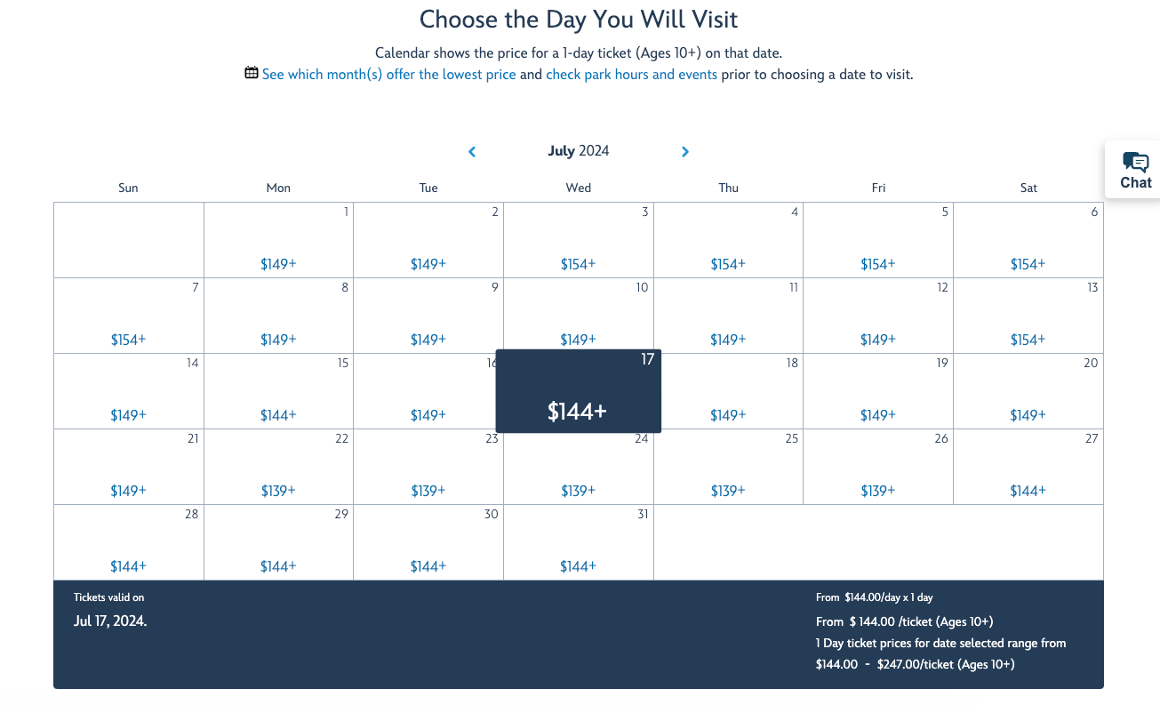
Doing so will let you get significantly more bang for your points (or dollars) than taking multiple short Disney trips — unless you're shopping for a Disney annual pass (which isn't a bad strategy if you plan to visit multiple times a year). Single-day, one-park tickets to Disney World range from $109 to $189. However, your per-day cost on a longer Disney trip of up to 10 days can start as low as $62 per day at certain times of the year.

Related: These are the best times to visit Disney World

Park hopping, which involves visiting more than one theme park in a single day, brings the price of a one-day adult Disney World ticket to $187 (plus tax), so you're looking at a real chunk of change ... or points.

How to redeem points for Disney tickets

If you're looking for a magical way to get outsize value when using your points for Disney tickets (as you might when redeeming airline miles for a first-class ticket ), we have some bad news. It's generally impossible to get a lucrative return when redeeming points for Disney tickets.

Instead, the best ways to redeem points for Disney tickets are by redeeming them at a fixed rate or via a cash-back card .

Related: How to rent Disney Vacation Club points and save hundreds of dollars on your vacation

That said, the best use for your points is the one that makes you happy. If Disney is your happy place, your points can unlock the gates for your visit.

Redeem Bilt Points for Disney tickets

Bilt Rewards is one of the best options for securing tickets to Disney.

With Bilt Rewards and the Bilt Mastercard® (see rates and fees ), you can earn points that be redeemed for Disney tickets directly in the activities section of the Bilt travel portal at a rate of 1.25 cents per point. This is a better return per point than most of the other options we'll go through. Cardholders must use the card five times each statement period to earn points (see rewards and benefits ).

While there are more valuable ways to redeem Bilt points with transfer partners, using Bilt Rewards points for Disney tickets is pretty solid. Also, if you take advantage of Bilt's monthly Rent Day offers, you can double your earnings on things like dining and give your points balance a boost.

In the example above, Bilt's travel booking site charges 11,570 points, or $144.62, for a one-day ticket to the Magic Kingdom on Aug. 20, while Disney charges $137.39 directly. Bilt's price includes a 5% convenience fee, so you will pay more in that case to use your points, but it's still one of the better uses of points for Disney tickets.

TPG founder Brian Kelly is a Bilt adviser and investor.

Redeem Chase points for Disney tickets

Three-day and longer Walt Disney World tickets can occasionally be found in the Chase Travel℠ portal . We spotted them as recently as early 2024, though they've since magically disappeared from the Chase site as of this update.

When available, you can redeem Chase Ultimate Rewards points for Disney tickets, cruises, resorts and vacation packages at 1.25 cents each if you hold a Chase Sapphire Preferred® Card or 1.5 cents each if you have a Chase Sapphire Reserve® . As is the case with Bilt, prices are slightly higher than if you just purchase directly from Disney.

With the Chase Sapphire Reserve, you can use the card's $300 annual travel credit toward Disney tickets as long as it codes as a travel charge. Since Disney tickets don't normally register as a travel charge, consider buying your tickets from a certified third-party seller like Undercover Tourist . As a bonus, some of the tickets available via Undercover Tourist cost a bit less than buying directly with Disney (though some tickets for shorter trips are more expensive).

Related: The best credit cards for your Disney vacation

Redeem travel points and miles for Disney tickets — with a catch

Like Bilt Rewards and Chase Ultimate Rewards , you can transfer Capital One miles from the Capital One Venture Rewards Credit Card and the Capital One Venture X Rewards Credit Card to hotel and airline partners . However, you can also redeem Capital One miles at a fixed rate of 1 cent each toward travel purchases made using the card.

The catch with this redemption method is that Disney tickets purchased directly from Disney don't typically code as a travel charge if purchased by themselves. As is the case with Chase, Disney tickets typically don't code as travel (unless you purchase a larger hotel-and-ticket vacation package). You'll want them to code that way if you want to offset costs by redeeming Capital One miles, so your best bet is to purchase your admission from a third-party site like Undercover Tourist.

If you do buy your tickets with a method that labels your purchase as a travel charge, you could use the 75,000-mile welcome bonus that you can earn after spending $4,000 on the Venture Rewards card in the first three months of having the card as $750 toward a Disney trip.

Related: The best Disney World hotels for your stay

Redeem flexible points against the charge

With some of the other credit card programs, the best you can do is earn cash-back rewards that could be used to offset the cost of Disney tickets — or anything else for that matter.

For example, Bank of America Preferred Rewards® points, which can be earned from the Bank of America® Premium Rewards® credit card , are worth 1 cent each. This card awards up to 2.625 points per dollar spent on non-bonus transactions and 3.5 points per dollar spent on travel and dining purchases if you've unlocked the Diamond tier of the Preferred Rewards program (which is based on the total amount of assets you have deposited with Bank of America and/or Merrill accounts).

If you are in that preferred earnings tier, it's just about the most rewarding cash-back card on the market.

The welcome bonus is now 60,000 points after spending $4,000 in the first 90 days of account opening. That has a $600 cash equivalent value that you could use to give yourself a statement credit, essentially offsetting the cost of the Disney tickets charged to that card.

What about the Disney Visa Card?

It's logical to wonder why, 1,000 words into the story, the namesake Disney® Visa® Card has yet to appear if you want to use points for a Disney vacation.

There are technically two versions of the Disney Visa. The no-annual-fee Disney Visa earns a simple 1% back on all card purchases in the form of Disney Rewards Dollars you can use at Disney.

Then there's the Disney® Premier Visa® Card , which has a $49 annual fee. It earns 5% back on card purchases made directly at DisneyPlus.com, Hulu.com and ESPNPlus.com, 2% back on purchases at gas stations, grocery stores, restaurants and most domestic Disney locations, and 1% back everywhere else.

In both cases, the Disney Rewards Dollars you earn can be used toward expenses at the Disney parks, on a Disney cruise, etc. This means that it's not a bad option if you want to rack up rewards for a Disney trip — especially if you lock in a good sign-up bonus, which we've seen as high as $400 on the Disney Visa Premier.

There are some cool perks and discounts that come with the cards, but they aren't the absolute best options for maximizing your ongoing spending to earn a future Disney vacation.

Related: Are the Disney Visa credit cards worth it?

Bottom line

It takes time and a concerted effort to build up enough points for a family's worth of Disney tickets. However, strategically using one or more big credit card sign-up bonuses can help turn a dream Disney trip into a more wallet-friendly reality.

For example, getting $750 in value toward your trip from the current bonus on the Capital One Venture Rewards Card and another $600 from the current welcome bonus on the Bank of America® Premium Rewards® credit card can give you a nice head start if you don't want to pay cash for Disney tickets.

If you have more time to stockpile points, then the Bilt Mastercard is a great option to have in your wallet since Bilt Rewards points are worth 1.25 cents each for Disney tickets. However, it currently doesn't have a welcome bonus for new cardholders.

Getting the Chase Sapphire Reserve and earning its 75,000-point welcome bonus (after you spend $4,000 in the first three months) could get you close to two three-day adult tickets as long as they are available in the Chase Travel portal.

While mathematically there are more economical applications for reward points than Disney ticket purchases, the best use of points is always the one that makes your travel dreams come true. So, if Disney is what you want for a future points-fueled trip, you can make that dream come true.

CmoorepetsTravel

Location & Hours

Suggest an edit

Round Rock, TX 78664

You Might Also Consider

You Can Leave

You Can Leave offers petsitting services, overnight in-home dog sitting, overnight in-home cat sitting, pet drop-in services, dog walking, notary services, poop scooping, plant watering, mail collection, in-home bird sitting, Pet… read more

in Pet Sitting, Dog Walkers

Sit Means Sit South Austin

24.2 miles away from CmoorepetsTravel

Sit Means Sit Dog Training Austin provides advanced obedience training that results in happy, confident and obedient dogs as well as happy, confident and satisfied owners. Unlike other trainers, we equip you to continue your dog's… read more

in Pet Training

Cedar Park Pet Sitting Services

John D. said "We had arranged with a work friend of my spouse to house sit and care for our two Boston Terriers while we went off for a week this summer. Long story short, the friend had two dogs of her own and I set up a 'meet and greet' with…" read more

in Pet Sitting

Recommended Reviews

1 star rating Not good
2 star rating Could’ve been better
3 star rating OK
4 star rating Good
5 star rating Great

Select your rating

Overall rating

Outstanding Pet Transport Service! I cannot recommend Cmoorepetstravel enough! They facilitated the seamless transportation of my new furry family member from Texas to California, and I couldn't be happier with the experience. From start to finish, their communication was exceptional, keeping me informed every step of the way. The care they provided for my pet was top-notch, ensuring his comfort and safety throughout the journey. Despite the long distance, they managed to transport my dog in just a little over one day, which was incredibly impressive. Everything about the process was amazing, from the professionalism of their team to the attention to detail in handling my pet's needs. If you're in need of pet transportation services, look no further than Cmoorepetstravel. They exceeded all my expectations, and I am immensely grateful for their outstanding service. Thank you for making the journey stress-free and delivering my beloved pet safely into my arms!

Such a great pet transportation company. I searched for a way to get a puppy to be transported across the US. I had looked into flying and picking up myself, having a company fly with the puppy from the breeder and ground transportation. After weighing all the options, ground transportation seemed the most cost-effective. After receiving multiple bids, Cmoorepets was the best option. Not knowing much about this method of travel, I was reliant on the Facebook page and the reviews that were on the page. I messaged the company and quickly received a quote. The setup process was very easy. I gave the pickup date and location and drop-off location. The payment was 1/2 on pickup and 1/2 at drop-off. A group text was setup between us, the breeder and the driver(Courtney-owner) and her co-driver(Christian-brother). We received many text messages and pictures along the way with location and updated estimated arrival times. This was such a great experience, I highly recommend this outfit if you are in need of transporting a pet. They are friendly, courteous, and trustworthy. I am thankful that in this day and age that there are companies that can be trusted with our most precious cargo.

Stay as far away from this company as possible!! They showed up at my house and approached me in a combative, threatening manner, getting in my face and trying to bully me. We had a disagreement about price because they kept pushing back my dogs arrival time by entire days so they could swing halfway across the country in the wrong direction to add extra stops and keep my dog in a van for 6 days. All they care about is money. When I came outside to get my dog, they wouldn't let me get him out of the car. HE LITERALLY ZIP TIED THE CRATE SHUT IN 3 PLACES and held my dog hostage, getting in my face saying give him the money NOW or I couldn't have my dog. I had to call the police. I had to take my dog to the emergency vet for fluids. He was dehydrated and constipated and severely stressed. They were nasty and argumentative in their communications and anything you say or do, they threaten legal action. They claim no one else ever complained about them being 3 days late to deliver a dog, but I talked to another rescue that dealt with them who had a similar experience. MOST UNPROFESSIONAL COMPANY EVER. Spend the extra money to work with a company who will respect you & your pet!

Our business specializes in superior customer service and satisfaction. We provide your pet(s) with the best grooming experience and we will make sure to meet and exceed your expectations 100% of the time. You do not need to leave… read more

in Pet Groomers

Suds and Pups

Suds and Pups Mobile Grooming - A fresh approach to pet comfort and convenience. read more

Browse Nearby

Restaurants

Cat Boarding

House Sitters

Other Pet Transportation Nearby

Find more Pet Transportation near CmoorepetsTravel

Related Cost Guides

Animal Shelters

Dog Walkers

Emergency Pet Hospital

Holistic Animal Care

Pet Photography

Pet Transportation

Veterinarians

5 More Cost Guides

IMAGES

VIDEO

Travel cost method
Transportation Model
The Travel-Cost Method! Environmental Valuation! #environmentaleconomics #ecojosh
GROUP 9 : TRAVEL COST METHOD
ANALISIS TRAVEL COST METHOD
Economic Valuation of Environmental Goods and Services

COMMENTS

Travel Cost Method
The travel cost method is used to estimate economic use values associated with ecosystems or sites that are used for recreation. The method can be used to estimate the economic benefits or costs resulting from: changes in access costs for a recreational site. elimination of an existing recreational site. addition of a new recreational site.
Travel cost analysis
The travel cost method of economic valuation, travel cost analysis, or Clawson method is a revealed preference method of economic valuation used in cost-benefit analysis to calculate the value of something that cannot be obtained through market prices (i.e. national parks, beaches, ecosystems).
Chapter 15: Environmental Valuation: The Travel Cost Method
The advantage of the CVM over some other approaches (e.g., Travel Cost Method, Hedonic Price Method, Choice Experiment) is the fact that it is more clear and comprehensible (see also Fatahi ...
Travel cost method
The Travel Cost Method (TCM) is one of the most frequently used approaches to estimating the use values of recreational sites. The TCM was initially suggested by Hotelling [1] and subsequently developed by Clawson [2] in order to estimate the benefits from recreation at natural sites. The method is based on the premise that the recreational ...
The travel cost method: a valuable tool for organizers quantifying the
A methodological approach to evaluate the value of EE is the travel cost method (TCM), which is a non-market valuation method in the field of environmental economics that uses travel data to determine what individuals are willing to pay to access a site of interest. Few studies have addressed the value of EE in this way.
PDF Chapter 15. Travel Cost Method of Valuing Environmental Amenities
The travel cost method is simple, not terribly controversial, and has a great deal of appeal to many people, since it is based on actual behavior. Moreover, this method can often be. 5 As with the survey methods discussed earlier, there are inevitably issues of survey design, selectivity bias,
Valuing the Recreation Uses of Natural Resources: The Travel Cost Method
The travel cost model (TCM) of recreation demand is a survey-based method that was developed to estimate the recreation-based use value of natural resource systems. The TCM may be used to estimate the value of. changes in the quality of recreation sites or natural resources systems (Freeman 2003).
Environmental Valuation: The Travel Cost Method
The travel cost method estimates the economic value of recreational sites or other concentrated environmental amenities (e.g., wildlife observation) by looking at the full travel costs (time, out of pocket, and any applicable fees) of visiting the sites. In existence since a letter written in 1949 from Harold Hotelling to the director of the ...
The Travel Cost Model
The Hedonic Travel Cost Method. Review of Economics and Statistics 66:427-433. Google Scholar Burt, O., and D. Brewer. 1971. Estimation of net Social Benefits from Outdoor Recreation. Econometrica 39(5):813-828. Google Scholar Chen, H. Z., and S. R. Cosslett. 1998. Environmental Quality Preference and Benefit Estimation in Multinomial ...
Travel Cost Models
The earliest travel cost models, dating from the late 1950s and into the 1960s, used "zonal" data and followed a method proposed by Hotelling ().Geographic zones were defined around a single recreation site.
Valuation of Ecosystem Services: Travel Cost Method
This video is a part of Conservation Strategy Fund's collection of environmental economics lessons and was made possible thanks to the support of Jon Mellber...
PDF TRAVEL COST METHOD (TCM)
3 TCM Travel cost method (TCM) is one of the popular methods used falls under the revealed preference approach to value non-priced or non-market good The other two approaches are: market-based and stated preference approach This approach is based on the assumption that the non- marketed good or service affect preferences expressed by consumers
PDF Travel Cost Method
travel time - Assume Zone 0 = zero travel distance and time - Multiply average travel distance for each zone by standard cost per mile (£0.3 per mile) - Multiply average travel time for each zone by the cost of time (e.g. average hourly rate, £9/hour or £0.15/minute) - Add travel and time cost together
Travel-cost method
The travel-cost method (TCM) is used for calculating economic values of environmental goods. Unlike the contingent valuation method, TCM can only estimate use value of an environmental good or service. It is mainly applied for determining economic values of sites that are used for recreation, such as national parks. For example, TCM can ...
The travel cost method and the economic value of leisure time
The travel cost method and the economic value of leisure time. January 1, 2004. Recent estimates of high values for tourist related recreation USA amenity values indicate that allocation of basic water and terrestrial resources to recreation activities should be given precedence over conventional market oriented activities that often degrade or ...
Travel-cost method for assessing the monetary value of recreational
Total travel cost: The increase in total travel costs, TC i, negatively affects the log persontrips' frequency (β ̂ = − 0.006), as expected from the travel-cost method. That means, for each 1 TL increase in total travel cost per person, the expected log count of the persontrips decreases by 0.006 while holding all other variables in the ...
PDF An examination of sources of sensitivity of consumer surplus estimates
2. Methods 2.1. The travel cost method (TCM) When an individual makes a trip to engage in a form of recre-ation, that person is spending time and money to "produce" the trip. This creates an "implicit market" for the environmental ame-nity associated with the trip. The most obvious market purchase
Environmental Valuation: The Travel Cost Method
The design of this work is to estimate the recreational value and to establish functional relationship between travel cost and visitation of Lawachara National Park (LNP) in Bangladesh. This study employed zonal approach of the travel cost method. The work is grounded on a sample of 422 visitors of the LNP. Results showed that the total value ...
The Individual Travel Cost Method with Consumer-Specific Values of
3.3 Travel Cost Method with Consumer-Specific Values of Travel Time Savings. In this section we present the estimation results of 5 travel cost models with different assumptions with respect to respondents' VTTS. Generally, visitor $i$ 's expected number of trips can be calculated as:
(PDF) Measuring Recreational Value Using Travel Cost Method (TCM): A
Travel Cost Method (TCM): A Number of Issues and Limitations. International Journal of Academic Research in Business and Social Sciences , 8 (10), 1381 - 1396.
Chapter 13
Chapter 13. Chapter 13. Revealed Preference MethodsNonmarket Valuation Methods. Travel Cost Method. Most applications of the travel cost method (TCM) have been to value recreational sites. Suppose that we want to estimate the value of a particular recreational site. We expect that the quantity of visits demanded by an individual depends on its ...
Travel Cost Method
The travel cost method involves collecting data on the costs incurred by each individual in travelling to the recreational site or amenity. This 'price' paid by visitors is unique to each individual, and is calculated by summing the travel costs from each individuals original location to the amenity. By aggregating the observed travel costs ...
Methods Used for the Environmental Valuation (With Diagram)
The travel-cost method is of limited value if congestion is a problem. Small changes affecting recreational quality may be difficult to evaluate using this method. 3. The basic assumption of travel-cost method is that consumers treat increase in admission fees as equivalent to increase in travel cost. This is subject to question.
How to use points to buy Disney tickets
In the example above, Bilt's travel booking site charges 11,570 points, or $144.62, for a one-day ticket to the Magic Kingdom on Aug. 20, while Disney charges $137.39 directly. Bilt's price includes a 5% convenience fee, so you will pay more in that case to use your points, but it's still one of the better uses of points for Disney tickets.
CMOOREPETSTRAVEL
2 reviews and 4 photos of CMOOREPETSTRAVEL "Such a great pet transportation company. I searched for a way to get a puppy to be transported across the US. I had looked into flying and picking up myself, having a company fly with the puppy from the breeder and ground transportation. After weighing all the options, ground transportation seemed the most cost-effective.