round trip time estimation

What Is Round Trip Time?

Last updated: March 18, 2024

1. Introduction

Networked communications are complex, and keeping the quality of connections is challenging for network operators and administrators. To do that, network operators execute several monitoring processes to analyze the results and find the proper actions to improve the network. In this context, several metrics are measured , such as throughput, packet loss, jitter, and round trip time.

In this tutorial, we’ll particularly study the Round Trip Time (RTT).  Initially, we’ll have a brief review on what is propagation time. Thus, we’ll in-depth understand the concept of round trip time, understanding how it works, and which events can typically vary its value. So, we’ll check some strategies to reduce the RTT. Finally, we’ll understand the similarities and differences between RTT and ping results.

2. Propagation Time

One of the most relevant components of RTT is propagation time.  In networking, propagation time means the total length of time that a signal takes to be sent from the source to the destination. We can also call the propagation time of one-way delay or latency.

A characteristic of propagation time is that there is no guarantee different sending processes of the same packet from the same source to the same destination present the same propagation time.

The following figure depicts the central notion of propagation time:

It is relevant to highlight the propagation time from the first machine to the second machine and the propagation time from the second machine to the first one, which can differ.

3. Round Trip Time

The RTT is the time between sending a message from a source to a destination (start) and receiving the acknowledgment from the destination at the source point (end).  We can also see RTT referred to as Round Trip Delay (RTD).

Sometimes, the acknowledgment is sent from the destination to the source almost immediately after the latter receives a message. Thus, the processing time at the destination point is negligible. In this way, the RTT consists of the propagation time from the source to the destination ($PT_m$) plus the propagation time from the destination to the source ($PT_a$).

A common misconception is assuming that the RTT is two times the propagation time from a source to a destination. However, the response message (acknowledgment) can have a different propagation time to arrive at the source point. It may occur due to a bottleneck in the network or different routes taken, for example.

Finally, another relevant characteristic of RTT is measuring it in the highest network layer possible. Thus, if we use protocols such as HTTPS , we may have some extra time to decrypt the message before sending the acknowledgment message. This additional time composes the RTT.

The following figure illustrates the measured times composing the RTT:

It is important to note that we measure RTT from the perspective of the message source (sender). Thus, RTT is pretty useful for getting some insights about, for example, the quality of service and experience of users of network-provided applications.

3.1. Managing the Round Trip Time

Several factors vary the RTT taking into account a particular source. Among the most prominent of them, we can cite the following ones:

• Existence of Network Bottlenecks : an overloaded network increases the RTT since it may incur some extra queueing, processing, and transmission times for packets being processed and forwarded by network functions
• Physical Distance Between Source and Destination : large physical distances between a source and destination result, at least, in more cables (or other transmission mediums) on which a message goes thorough. But it can also result in more hops and extra network function processing
• Transmission Technologies Employed : data transmission over optical fiber has different characteristics than doing that through copper cables, which, in turn, differs from a wireless medium. The transmission technology employed may directly impact the RTT

Some techniques can reduce the RTT when requesting and retrieving a network-provided resource. Let’s see some of them:

• Track the connections : constantly monitoring the RTT of connections is essential to understand how to improve it. According to the obtained results, we can optimize the networking routes and simplify the exchanged data and the operations done in the system
• Refactor the system : reducing the number of unique hostnames may save time with DNS operations; moreover, keeping the system updated and free from broken lists or pages helps to not waste time
• Bring resources near users : providing resources through CDN is a great option to reduce the propagation delay and, consequently, the RTT; for web pages, enabling browser caching can also be efficient for that

Minimizing the global RTT of a system is a difficult task. Different users have different experiences in retrieving data or executing operations due to their geographical positions and the conditions of the networking routes employed. So, system administrators should make it the most efficient possible in opening connections and responding to requests and, if possible, make resources available near end-user-dense regions.

4. RTT vs. Ping

Ping stands for Packet Internet-Network Groper and is a simple network software tool. This tool employs the Internet Control Message Protocol (ICMP), sending echo requests from a source point and waiting for echo replies from the destination system.

In this way, Ping can check the destination system reachability, provide packet loss statistics, report some errors, and calculate the minimum, average, and maximum RTT.

So, the question is: can we use ping to calculate RTT for any system?

The answer to the previous question is no. As previously stated, ping works with ICMP (which is a network layer protocol). But, RTT always is measured in the highest layer that a system operates on. So, we can not use ping to precisely measure the RTT of an HTTPS system, for example.

However, although not a synonym in every scenario, ping provides a pretty good estimation of RTT and can be generically used to measure it when high precision on the results is not a strict requirement.

5. Conclusion

In this article, we explored the Round Trip Time.  First, we reviewed the concept of propagation time, which is crucial to understand RTT. Thus, we specifically investigated RTT by presenting its fundamentals, the most common factors that impact its value, and techniques to reduce the average RTT for accessing particular network-provided resources and systems. Finally, we show the similarities and differences between ping-based time measurements and RTT.

We can conclude that RTT is a pretty relevant metric for network monitoring.  RTT provides valuable insights into the quality of service and experience, thus working as a significant piece of information for improving network-provided resources and systems.

Written by Vasilena Markova • September 27, 2023 • 12:58 pm • Internet

Round-Trip Time (RTT): What It Is and Why It Matters

Round-Trip Time (RTT) is a fundamental metric in the context of network performance, measuring the time it takes for data packets to complete a round trip from source to destination and back. Often expressed in milliseconds (ms), RTT serves as a critical indicator for evaluating the efficiency and reliability of network connections. In today’s article, we dive into the concept of RTT, exploring how it works, why it matters in our digital lives, the factors that influence it, and strategies to enhance it. Whether you’re a casual internet user seeking a smoother online experience or a network administrator aiming to optimize your digital infrastructure, understanding this metric is critical in today’s interconnected world.

Table of Contents

What is Round-Trip Time (RTT)?

Round-Trip Time is a network performance metric representing the time it takes for a data packet to travel from the source to the destination and back to the source. It is often measured in milliseconds (ms) and is a crucial parameter for determining the quality and efficiency of network connections.

To understand the concept of RTT, imagine sending a letter to a friend through the postal service. The time it takes for the letter to reach your friend and for your friend to send a reply back to you forms the Round-Trip Time for your communication. Similarly, in computer networks, data packets are like those letters, and RTT represents the time it takes for them to complete a round trip.

How Does it Work?

The concept of RTT can be best understood by considering the journey of data packets across a network. When you request information from a web server, for example, your device sends out a data packet holding your request. This packet travels through various network devices in between, such as routers and switches, before reaching the destination server. Once the server processes your request and prepares a response, it sends a data packet back to your device.

Round-Trip Time is determined by the time it takes for this data packet to travel from your device to the server (the outbound trip) and then back from the server to your device (the inbound trip). The total RTT is the sum of these two one-way trips.

Let’s break down the journey of a data packet into several steps so you can better understand the RTT:

• Sending the Packet: You initiate an action on your device that requires data transmission. For example, this could be sending an email, loading a webpage, or making a video call.
• Packet Travel: The data packet travels from your device to a server, typically passing through multiple network nodes and routers along the way. These middle points play a significant role in determining the RTT.
• Processing Time: The server receives the packet, processes the request, and sends a response back to your device. This processing time at both ends also contributes to the Round-Trip Time.
• Return Journey: The response packet makes its way back to your device through the same network infrastructure, facing potential delays on the route.
• Calculation: It is calculated by adding up the time taken for the packet to travel from your device to the server (the outbound trip) and the time it takes for the response to return (the inbound trip).

Experience Industry-Leading DNS Speed with ClouDNS! 

Ready for ultra-fast DNS service? Click to register and see the difference!

Why does it matter?

At first look, Round-Trip Time (RTT) might seem like technical terminology, but its importance extends to various aspects of our digital lives. It matters for many reasons, which include the following:

• User Experience

For everyday internet users, RTT influences the sensed speed and responsiveness of online activities. Low Round-Trip Time values lead to a seamless experience, while high RTT can result in frustrating delays and lag during tasks like video streaming, online gaming, or live chats.

• Network Efficiency

Network administrators and service providers closely monitor RTT to assess network performance and troubleshoot issues. By identifying bottlenecks and areas with high RTT, they can optimize their infrastructure for better efficiency.

• Real-Time Applications

Applications that rely on real-time data transmission, such as VoIP calls, video conferencing, and online gaming, are highly sensitive to RTT. Low RTT is crucial for smooth, interruption-free interactions.

In cybersecurity, Round-Trip Time plays a role in detecting network anomalies and potential threats. Unusually high RTT values can be a sign of malicious activity or network congestion.

Factors Affecting Round-Trip Time (RTT)

Several factors can influence the metric, both positively and negatively. Therefore, understanding these factors is crucial, and it could be very beneficial for optimizing network performance:

• Distance: The physical distance between the source and destination plays a significant role. Longer distances result in higher RTT due to the time it takes for data to travel the network.
• Network Congestion: When a network experiences high volumes of traffic or congestion, data packets may be delayed as they wait for their turn to be processed. As a result, it can lead to packet delays and increased RTT.
• Routing: The path a packet takes through the network can significantly affect RTT. Efficient routing algorithms can reduce the time, while not-so-optimal routing choices can increase it.
• Packet Loss: Packet loss during transmission can occur due to various reasons, such as network errors or congestion. When lost, packets need to be retransmitted, which can seriously affect the Round-Trip Time.
• Transmission Medium: It is a critical factor influencing RTT, and its characteristics can vary widely based on the specific medium being used. Fiber optic cables generally offer low RTT due to the speed of light in the medium and low signal loss. In contrast, wireless mediums can introduce variable delays depending on environmental factors and network conditions.

How to improve it?

Improving Round-Trip Time (RTT) is a critical goal for network administrators and service providers looking to enhance user experiences and optimize their digital operations. While some factors affecting it are beyond our control, there are strategies and practices to optimize Round-Trip Time for a smoother online experience:

• Optimize Routing: Network administrators can optimize routing to reduce the number of hops data packets take to reach their destination. This can be achieved through efficient routing protocols and load balancing .
• Optimize Network Infrastructure: For businesses, investing in efficient network infrastructure, including high-performance routers and switches, can reduce internal network delays and improve RTT.
• Upgrade Hardware and Software: Keeping networking equipment and software up-to-date ensures that you benefit from the latest technologies and optimizations that can decrease RTT.
• Implement Caching: Caching frequently requested data closer to end-users can dramatically reduce the need for data to travel long distances. The result really helps with lowering RTT.
• Monitor and Troubleshoot: Regularly monitor your network for signs of congestion or packet loss. If issues arise, take steps to troubleshoot and resolve them promptly.

Discover ClouDNS Monitoring service!

Round-Trip Time (RTT) is the silent force that shapes our online experiences. From the seamless loading of web pages to the quality of our video calls, RTT plays a pivotal role in ensuring that digital interactions happen at the speed of thought. As we continue to rely on the Internet for work, entertainment, and communication, understanding and optimizing this metric will be crucial for both end-users and network administrators. By reducing it through strategies, we can have a faster, more responsive digital world where our online activities are limited only by our imagination, not by lag.

Hello! My name is Vasilena Markova. I am a Marketing Specialist at ClouDNS. I have a Bachelor’s Degree in Business Economics and am studying for my Master’s Degree in Cybersecurity Management. As a digital marketing enthusiast, I enjoy writing and expressing my interests. I am passionate about sharing knowledge, tips, and tricks to help others build a secure online presence. My absolute favorite thing to do is to travel and explore different cultures!

Related Posts

Ping Traffic Monitoring: Ensuring Network Health and Efficiency

March 28, 2024 • Monitoring

In an era where digital connectivity is the lifeline of businesses and individuals alike, maintaining optimal network performance is more ...

Leave a Reply Cancel reply

Your email address will not be published. Required fields are marked *

Recent Posts

• What is Backup DNS?
• BIND Explained: A Powerful Tool for DNS Management
• HTTP vs HTTPS: Why every website needs HTTPS today
• ccTLD – Building Trust and Credibility with Country-Specific Domains
• DDoS amplification attacks by Memcached
• Cloud Computing
• DNS Records
• Domain names
• Load balancing
• SSL Certificates
• Uncategorized
• Web forwarding
• DNS Services
• Managed DNS
• Dynamic DNS
• Secondary DNS
• Reverse DNS
• DNS Failover
• Anycast DNS
• Email Forwarding
• Enterprise DNS
• Domain Names

Home  >  Learning Center  >  Round Trip Time (RTT)  

Article's content

Round trip time (rtt), what is round trip time.

Round-trip time (RTT) is the duration, measured in milliseconds, from when a browser sends a request to when it receives a response from a server. It’s a key performance metric for web applications and one of the main factors, along with Time to First Byte (TTFB), when measuring  page load time  and  network latency .

Using a Ping to Measure Round Trip Time

RTT is typically measured using a ping — a command-line tool that bounces a request off a server and calculates the time taken to reach a user device. Actual RTT may be higher than that measured by the ping due to server throttling and network congestion.

Example of a ping to google.com

Factors Influencing RTT

Actual round trip time can be influenced by:

• Distance  – The length a signal has to travel correlates with the time taken for a request to reach a server and a response to reach a browser.
• Transmission medium  – The medium used to route a signal (e.g., copper wire, fiber optic cables) can impact how quickly a request is received by a server and routed back to a user.
• Number of network hops  – Intermediate routers or servers take time to process a signal, increasing RTT. The more hops a signal has to travel through, the higher the RTT.
• Traffic levels  – RTT typically increases when a network is congested with high levels of traffic. Conversely, low traffic times can result in decreased RTT.
• Server response time  – The time taken for a target server to respond to a request depends on its processing capacity, the number of requests being handled and the nature of the request (i.e., how much server-side work is required). A longer server response time increases RTT.

See how Imperva CDN can help you with website performance.

Reducing RTT Using a CDN

A CDN is a network of strategically placed servers, each holding a copy of a website’s content. It’s able to address the factors influencing RTT in the following ways:

• Points of Presence (PoPs)  – A CDN maintains a network of geographically dispersed PoPs—data centers, each containing cached copies of site content, which are responsible for communicating with site visitors in their vicinity. They reduce the distance a signal has to travel and the number of network hops needed to reach a server.
• Web caching  – A CDN  caches  HTML, media, and even dynamically generated content on a PoP in a user’s geographical vicinity. In many cases, a user’s request can be addressed by a local PoP and does not need to travel to an origin server, thereby reducing RTT.
• Load distribution  – During high traffic times, CDNs route requests through backup servers with lower network congestion, speeding up server response time and reducing RTT.
• Scalability  – A CDN service operates in the cloud, enabling high scalability and the ability to process a near limitless number of user requests. This eliminates the possibility of server side bottlenecks.

Using tier 1 access to reduce network hops

One of the original issues CDNs were designed to solve was how to reduce round trip time. By addressing the points outlined above, they have been largely successful, and it’s now reasonable to expect a decrease in your RTT of 50% or more after onboarding a CDN service.

Latest Blogs

Erez Hasson

May 17, 2024 5 min read

Grainne McKeever

May 8, 2024 3 min read

Apr 16, 2024 4 min read

Mar 13, 2024 2 min read

Mar 4, 2024 3 min read

Feb 26, 2024 3 min read

Feb 20, 2024 4 min read

Jan 18, 2024 3 min read

Latest Articles

• Network Management

173.1k Views

170.2k Views

155.5k Views

108.4k Views

102.6k Views

100.9k Views

60.2k Views

55.6k Views

2024 Bad Bot Report

Bad bots now represent almost one-third of all internet traffic

The State of API Security in 2024

Learn about the current API threat landscape and the key security insights for 2024

Protect Against Business Logic Abuse

Identify key capabilities to prevent attacks targeting your business logic

The State of Security Within eCommerce in 2022

Learn how automated threats and API attacks on retailers are increasing

Prevoty is now part of the Imperva Runtime Protection

Protection against zero-day attacks

No tuning, highly-accurate out-of-the-box

Effective against OWASP top 10 vulnerabilities

An Imperva security specialist will contact you shortly.

Top 3 US Retailer

• Open access
• Published: 26 March 2014

A machine learning framework for TCP round-trip time estimation

• Bruno Astuto Arouche Nunes 1 ,
• Kerry Veenstra 1 ,
• William Ballenthin 2 ,
• Stephanie Lukin 3 &
• Katia Obraczka 1  

EURASIP Journal on Wireless Communications and Networking volume  2014 , Article number:  47 ( 2014 ) Cite this article

6514 Accesses

26 Citations

1 Altmetric

Metrics details

In this paper, we explore a novel approach to end-to-end round-trip time (RTT) estimation using a machine-learning technique known as the experts framework . In our proposal, each of several ‘experts’ guesses a fixed value. The weighted average of these guesses estimates the RTT, with the weights updated after every RTT measurement based on the difference between the estimated and actual RTT.

Through extensive simulations, we show that the proposed machine-learning algorithm adapts very quickly to changes in the RTT. Our results show a considerable reduction in the number of retransmitted packets and an increase in goodput, especially in more heavily congested scenarios. We corroborate our results through ‘live’ experiments using an implementation of the proposed algorithm in the Linux kernel. These experiments confirm the higher RTT estimation accuracy of the machine learning approach which yields over 40% improvement when compared against both standard transmission control protocol (TCP) as well as the well known Eifel RTT estimator. To the best of our knowledge, our work is the first attempt to use on-line learning algorithms to predict network performance and, given the promising results reported here, creates the opportunity of applying on-line learning to estimate other important network variables.

1 Introduction

Latency is an important parameter when designing, managing, and evaluating computer networks, their protocols, and applications. One metric that is commonly used to capture network latency is the end-to-end round-trip time (RTT) which measures the time between data transmission and the receipt of a positive acknowledgment. Depending on how the RTT is measured (e.g., at which layer of the protocol stack), besides the time it takes for the data to be serviced by the network, the RTT also accounts for the ‘service time’ at the communication end points. In some cases, RTT measurement can be done implicitly by using existing messages; however, in several instances, explicit ‘probe’ messages have to be used. Such explicit measurement techniques can render the RTT estimation process quite expensive in terms of their communication and computational burden.

Several network applications and protocols use the RTT to estimate network load or congestion and therefore need to measure it frequently. The transmission control protocol, TCP, is one of the best known examples. TCP bases its error, flow, and congestion control functions on the estimated RTT instead of relying on feedback from the network. This pure end-to-end approach to network control is consistent with the original design philosophy of the Internet which keeps only the bare minimum functionality in the network core, pushing everything else to the edges. Overlays such as content distribution networks (CDNs) (e.g., Akamai [ 1 ]) and peer-to-peer networks also make use of RTT as a ‘network proximity’ metric, e.g., to help decide where to re-direct client requests. There has also been increasing interest in network proximity information from applications that run on mobile devices (e.g., smart phones) in order to improve the user’s experience.

In this paper, we propose a novel RTT estimation technique that uses a machine-learning based approach called the experts framework [ 2 ]. As described in detail in Section 3, the experts framework a uses ‘on-line’ learning, where the learning process happens in trials . At every trial, a number of experts contribute to an overall prediction, which is compared to the actual value of the RTT (e.g., obtained by measurement). The algorithm uses the prediction error to refine the weights of each expert’s contribution to the prediction; the updated weights are used in the next iteration of the algorithm. We contend that by employing the proposed prediction technique, network applications, and protocols that make use of the RTT do not have to measure it as frequently.

As an example application for the proposed RTT estimation approach, we use it to predict TCP’s RTT. Through extensive simulations and live experiments, we show that our machine learning technique can adapt to changes in the RTT faster and thus predict its value more accurately than the current exponential weighted moving average (EWMA) technique employed by most versions of TCP. As described in Section 2, TCP uses the RTT estimates to compute its retransmission time-out (RTO) timer [ 3 ], which is one of the main timers involved in TCP’s error and congestion control. When the RTO expires, the TCP sender considers the corresponding packet to be lost and therefore retransmits it. TCP relies on RTT predictions and measurements in order to set the RTO value properly. In TCP, the RTT is defined as the time interval between when a packet leaves the sender and until the reception, at the sender, of a positive acknowledgment for that packet.

If the RTO is too long, it can lead to long idle waits before the sender reacts to the presumably lost packet. On the other hand, if the RTO is set to be too aggressive (too short), it might expire too often leading to unnecessary retransmissions. Needless to say that setting the RTO is critical for TCP’s performance.

We can split the problem of setting TCP’s RTO into two parts. The first part is how to predict the RTT of the next packet to be transmitted, and the second is how the predicted RTT can be used to compute the RTO. In this paper, we focus on the first part of the problem, i.e., the prediction of the RTT; the second part of the problem, i.e., setting the RTO, is the focus of future work.

To estimate the RTT, we propose a new approach based on machine learning which will be described in detail in Section 3. Our experimental results show that RTT predictions using the proposed technique are considerably more accurate when compared to TCP’s original RTT estimation algorithm and the well-known Eifel [ 4 ] timer. We then evaluate how this increased accuracy affects network performance. We do so by running network simulations as well as live experiments. For the latter, we have implemented both our machine learning as well as the Eifel mechanism in the Linux kernel.

The remainder of this paper is organized as follows. Section 2 presents related work, including a brief overview of TCP’s original RTT estimation technique. In Section 3, we describe our RTT prediction algorithm. Section 4 presents our experimental methodology, where we describe the scenarios conceived for our simulation studies, discuss simulation parameters, and define metrics for performing evaluations. Sections 5 and 6, respectively, present our results from both simulation and live experiments. Finally, Section 7 concludes the paper and highlights directions for future work.

2 Related work

In this section, we present a brief overview of previous work on RTT estimation and later discuss some relevant machine learning applications.

2.1 TCP RTT estimation

TCP uses a time-out/retransmission mechanism to recover from lost segments. This time-out value needs to be greater than the current RTT to avoid unnecessary retransmissions; on the other hand, if it is too high, it will cause TCP to wait too long to react to losses and congestion. In Jacobson’s well-known work [ 3 ], two state variables EstimatedRTT and RTTVAR keep the estimate of the next RTT measurement ( SampleRTT ) and the RTT variation, respectively. RTTVAR is defined as an estimate of how much EstimatedRTT typically deviates from SampleRTT . EstimatedRTT is updated according to an EWMA given by Equation 1 , where α = 1 8 . RTTVAR is calculated using Equation 2 which is also an EWMA; this time of the difference between SampleRTT and EstimatedRTT with gain β typically set to 1 4 . Equation 3 sets the new value for the RTO as a function of EstimatedRTT and RTTVAR , where K is usually 4.

Most current variants of TCP also implement Karn’s Algorithm [ 5 ], which ignores the SampleRTT corresponding to retransmissions. Another consideration is TCP’s clock granularity. In several TCP implementations, and also in the simulation tool used in this work, the clock advances in increments of ticks commonly set to 500 ms, and the RTO is bounded by RTO min =2· ticks and RTO max =64· ticks b .

In prior work, a number of approaches have been proposed to estimate TCP’s RTT. Trace-driven simulations reported in [ 6 ] to evaluate different RTT estimation algorithms show that the performance of the estimators is dominated by their minimum values and is not influenced by the RTT sample rate [ 6 ]. This last conclusion was challenged by the Eifel estimation mechanism [ 4 ], one of the most cited alternatives to TCP’s original RTT estimator; Eifel can be used to estimate the RTT and set the RTO. Eifel’s proponents identify several problems with TCP’s original RTT estimation algorithm, including the observation that a sudden decrease in RTT causes RTTVAR and consequently the RTO to increase unexpectedly c . As it will become clear from the experimental results presented in Subsection 6.3, our approach is able to follow quite closely any abrupt changes in the RTT and outperforms both TCP’s original RTT estimator as well as that of Eifel’s.

Another notable adaptive TCP RTT estimator was proposed in [ 7 ]. It uses the ratio of previous and current bandwidth to adjust the RTT. In [ 8 ], a TCP retransmission time-out algorithm based on recursive weighted median filtering is proposed. Their simulation results show that for Internet traffic with heavy tailed statistics, their method yields tighter RTT bounds than TCP’s original RTT computation algorithm. Leung et al. present work that focuses on changing RTO computation and retransmission polices, rather than improving RTT predictions [ 9 ].

2.2 Selected machine learning applications

Machine learning has been used in a number of other applications. Helmbold et al. use an experts framework algorithm to predict hard-disk drive’s idle time and decide when to attempt to save energy by spinning down the disk [ 10 ]. For this problem, the cost of making a bad decision (i.e., when spinning the disk down and back up costs more than simply leaving it on) is very well defined since the decision of spinning down the disk does not affect the length of the next idle time.

Unlike the spin-down example, when predicting the RTT, every prediction causes the next RTT to be set to a different value and that influences every event that happens thereafter. Thus, the problem of defining the cost of a bad RTT prediction is not as straightforward. Our solution to this problem is discussed in Section 3.

Moreover, in the spin-down cost problem, the traces used in the evaluation were ‘off-line’ traces, i.e., traces captured from live runs and later on used as input to the algorithms being evaluated. In the case of the spin-down problem, there is no problem in using off-line traces since the algorithm’s estimations do not influence the outcome of the next measurement. In the case of TCP RTT estimation, however, as previously discussed, since the RTT estimations influence TCP timers and these timers affect the outcome of the next RTT measurement, off-line traces can be used to set and tune parameters of the algorithm, but they are not suitable for evaluating the performance of the system. The work presented in [ 8 , 9 , 11 , 12 ] on RTT estimation compares their solution against TCP’s original RTT estimation algorithm, but they base their evaluation on off-line traces.

Machine learning techniques have not been commonly employed to address network performance issues. The work described in [ 13 ] is a notable exception and proposes the use of the stochastic estimator learning algorithm (SELA) to address the call admission control (CAC) problem in the context of asynchronous transfer mode (ATM) networks. Their goal was to predict in ‘real time’ if a call request should be accepted or not for various types of traffic sources. Simulation results show the statistical gain exhibited by the proposed approach compared to other CAC schemes. Another SELA-based approach, this time, applied to QoS routing in hierarchical ATM networks was proposed in [ 14 ]. In this approach, learning algorithms operating at various network switches determine how the traffic should be routed based on current network conditions. In the context of WiMax networks, a cross-layer design approach between the transport and physical layers for TCP throughput adaptation was introduced in [ 15 ]. The proposed approach uses adaptive coding and modulation (ACM) schemes.

Mirza et al. propose a throughput estimation tool based on support vector regression modeling [ 16 ]. It predicts throughput based on multiple real-value input features. However, to the best of our knowledge, to date, no attempt to use on-line learning algorithms to predict network conditions has been reported.

3 Proposed approach

In this section, we present the fixed-share experts algorithm as a generic solution for on-line prediction. Later, we describe its application to the problem of predicting the RTT of a TCP connection.

3.1 The fixed-share experts algorithm

Our RTT prediction algorithm is based on the fixed-share experts algorithm [ 2 ] which uses ‘on-line learning’ based on the predictions of a set of fixed experts denoted by { x 1 , …, x N }. In on-line learning, the learning process happens in trials. Figure 1 illustrates these trials and the algorithm itself. Under the fixed-share experts algorithm, at every trial t , the algorithm receives the predictions x i   ∀   i   ∈  {1, …, N } from a total of N experts and uses them to output a master prediction ŷ t . After trial t is completed, the ‘ground truth’ value y t becomes known and is used to compute the estimation error based on a loss function , L . The estimation error computed at trial t for every expert i is thus given by L i , t ( x i , y t ) which is used to update a set of weights . The next prediction for trial t +1 is calculated using this new set of weights denoted by W t +1, i  = { w t +1,1 , …, w t +1, i , …, w t +1, N }.

Graphical representation of the general fixed-share experts algorithm for RTT estimation.

The weight w t , i should be interpreted as a measurement of the confidence in the quality of the i th expert’s prediction at the start of trial t . In the initialization of the algorithm, we make w 1 , i = 1 N , ∀ i ∈ { 1 , … , N } . The algorithm updates the experts’ weights at every trial after computing the loss at trial t by multiplying the weight of the i th expert by e - η L i , t ( x i , y t ) . The learning rate η is used to determine how fast the updates will take effect, dictating how rapidly the weights of misleading experts will be reduced.

After updating the weights, the algorithm also ‘shares’ some of the weight of each expert among other experts. Thus, an expert who is performing poorly and had its weight severely compromised can quickly regain influence in the master prediction once it starts predicting well again. The amount of sharing can be changed by using the α parameter, called the sharing rate . This allows the algorithm to adapt to ‘bursty’ behavior. Indeed, in Section 5, we use, among others, bursty traffic scenarios to evaluate the performance of our algorithm.

Algorithm 1 summarizes the steps involved in our fixed-share experts algorithm. The first line in the algorithm summarizes the algorithm’s parameters, namely: (1) the learning rate η , which we define as a positive real number, and (2) the sharing rate α , a real number between zero and one that dictates the percentage of the weights shared at every trial. In our approach, expert weights are initialized uniformly, which is what is described in the ‘Initialization’ step of Algorithm 1. The basic four steps of our fixed-share experts algorithm are also summarized in Algorithm 1 (and in Figure 1 ). In step 1, the prediction defined as a the weighted average over the individual predictions x i of every i th expert is computed. The loss function is computed in step 2 and is used in step 3 to penalize and decrease the weights of the experts that are not performing well, and in step 4, experts share their weight based on the sharing rate α .

In [ 2 ], the basic version of the experts framework is presented along with bounds for different loss functions. The algorithm is also analyzed for different prediction functions, including the weighted averaging we use. The implementation described in this paper, with the intermediate pool variable, costs O (1) time per expert per trial.

3.2 Applying experts to TCP’s RTT prediction

To apply the proposed algorithm to TCP’s RTT-prediction problem, the experts predictions x i shown in Algorithm 1 serve as predictions for the next RTT measured. y t is the RTT value at the present trial, equivalent to the SampleRTT in the original TCP RTT estimator. ŷ t is the output of the algorithm, or in other words, the RTT prediction itself, equivalent to the EstimatedRTT in the original TCP RTT predictor, mentioned in Section 2.

Algorithm 1 Fixed-share experts algorithm

We want the loss function L i , t ( x i , y t ) to reflect the real cost of making wrong predictions. In our implementation (see Algorithm 1), the loss function has different penalties for overshooting and undershooting the RTT estimate as they have different impact on the system’s behavior and performance. An underestimate of the RTT will result in an RTO computation that is less than the next measured RTT, causing unnecessary timeouts and retransmissions. We thus employ the following policies: if the measured RTT y t is higher than the expert’s prediction x i , then it means that this expert is contributing to a spurious timeout and should be penalized more than other experts that overshoot within a given threshold. Big over-shooters are more severely penalized. The challenge here is identifying the appropriate cost for miss-predicting the RTT. The cost could be simply the difference between prediction and measurement, or a factor thereof. Exploring other loss functions for the TCP RTT estimation problem is the subject of future work.

Setting the value x i of the experts is referred to as setting the experts spacing . To space the experts is to determine the experts’ values and their distribution within the prediction domain. When predicting RTTs, the experts should be spaced between RTT min and RTT max , defined in some TCP implementations (including the one in the network simulator we used in our experimental evaluation) to be 1 and 128 ticks, respectively. Based on observations of several RTT datasets, we concluded that the majority of the RTT measurements are concentrated in the lower part of this interval. For that reason, we found that spacing the experts exponentially in that interval, instead of uniformly (or linearly), leads to better predictions. The exponential function used in our implementation of the Fixed-Share Experts approach is x i = RTT min + RTT max · 2 ( i - N ) 4 . The 1 4 multiplicative factor in the exponent of the spacing function was experimentally chosen to smooth out its growth. This increases the difference between the experts and generates diversity among them, which increases predictions’ granularity and accuracy.

Another consideration is that the algorithm, as stated in Algorithm 1, will continually reduce the experts’ weights towards zero. Thus, in order to avoid underflow issues in our implementation, we periodically rescale the weights. Different versions of the multiplicative weight algorithmic family, including a mixing past approach that also mixes weights from past trials are discussed in [ 17 ]. However, the mixing past approach incurs higher space and time costs and thus was not considered in our work. Another sharing scheme known as variable-sharing was also considered in preliminary experiments, where the amount of shared weights to each expert was dependent of their individual losses. However, the additional complexity and cost of this scheme outweighed its benefits in terms of RTT estimation accuracy.

4 Experimental methodology

We conduct simulations using the QualNet [ 18 ] network simulation platform. In all experiments, unless stated otherwise, the simulation area is 1,500 m × 1,000 m and the simulated time is 25 min. The routing protocol used was AODV [ 19 ], and the medium access and physical layers defined at the IEEE 802.11.b [ 20 ] standard was used. The transmission radius was set to 100 m for all the nodes, which are initially placed in the simulation area uniformly distributed. On mobile scenarios, nodes move according to the random way point (RWP) mobility regime with 0 s of pause time and speed ranging between [1, 50] m/s. All nodes run file transmission protocol (FTP) applications to generate the TCP flows; TCP buffer size is the default TCP buffer size set to 16,384 bytes, and packet size is fixed at 512 bytes. For the reader convenience, we summarize the simulation parameters for all simulation scenarios in Table 1 . The value na is attributed to a given parameter in this table when it is not applicable . These and other simulation parameters, such as traffic patterns and number of flows will be discussed further in the following sections in a per-scenario basis.

In Section 5, we present results for a total of five simulation scenarios, which are summarized, along with their parameters, in Table 1 . The goal of having a variety of scenarios is to subject the proposed RTT estimation approach to a wide range of network conditions. Scenarios I and II represent ad hoc mobile networks composed of 20 and 10 nodes, respectively. These two scenarios differ from each other only in terms of node density. Scenario III is a static wireless network composed of 20 nodes uniformly distributed over the simulated network area. Scenario IV is also a 20-node mobile network, but the traffic pattern is different from scenarios I and II. In scenario IV, we also vary the mobility of the network by varying the nodes’ average speed. Finally, scenario V is a wired network composed of eight nodes, four on each side of a bottleneck link.

It is important to highlight that the mobile scenarios employed in our evaluation were used to evaluate the proposed RTT estimation technique under conditions that cause high variability and randomness in the network and thus in the RTT values. Following the RWP mobility regime, nodes move randomly causing data paths to break and new ones to be created which then results in high variability of the RTT. Our goal was then to ensure that our RTT estimator is able to adjust to high variability conditions and yield accurate RTT estimates.

We present our results in Section 5 using a number of performance metrics defined as follows:

Mean error on RTT prediction : absolute difference between the RTT prediction ŷ t and the measured RTT y t at trial t , averaged over all trials, defined as: 1 T ∑ t = 1 T | ŷ t - y t | . In the simulations, RTT is measured in ‘ticks’ of 500 ms. This value is equal to 4 ms in the real live experiments described in Section 6. The mean RTT prediction error metric is thus, also given in ‘ticks’.

Average congestion window size (cwnd) : the size in bytes of the congestion window at the TCP sender, averaged over all prediction trials, defined as: 1 T ∑ t = 1 T cwnd t , where c w n d t is the congestion window size measured at trial t .

Delivery ratio : ratio between total data packets received by the destination and data packets sent at the source, computed for every flow and averaged over all flows.

Percentage of retransmitted packets : ratio between retransmitted data packets and total data packets sent at every flow, averaged over all flows.

Goodput : total number of useful (data) packets received at the application layer divided by the total duration of the flow and averaged for every flow, giving a ratio of packets per second.

Following, we discuss the impact of the parameters in the accuracy of the proposed RTT prediction algorithm and justify the choice of values set to these parameters in our simulation evaluations.

4.1 Impact of experts framework parameters ( N,η,α )

We experimented with several combinations of the fixed-share algorithm parameters. The number N of experts affects the granularity over the range of values the RTT can assume. In our experiments, N >100 had no major impact on the prediction accuracy.

The learning rate η is responsible for how fast the experts are penalized for a given loss. We want to avoid values of η that are too low since it increases the algorithm’s convergence time; conversely, if η is too high, it forces the expert’s weights toward zero too quickly. If this is the case, then as weight rescaling kicks in, the algorithm assigns similar weights to all experts, making the algorithm’s master prediction fluctuate undesirably around the mean value of the experts’ guesses. We chose a learning rate in the interval 1.7 <  η  < 2.5 as it provides good prediction results for all the scenarios tested.

When sharing is not enabled, i.e., α  = 0, the outcome of the algorithm is given only by decreasing exponential updates, making it harder for the algorithm to follow abrupt changes in the RTT measurements: experts that experience prolonged poor performance lack influence because their weights have become too depreciated. In this case, it would take more trials so that these experts start gaining greater importance in the master prediction. Enabling full sharing ( α  = 1), similar weights are assigned to every expert, and the master prediction fluctuates close to a mean value among the experts guesses.

We present in more detail the simulation scenarios in the next section, highlighting the goals for every evaluation and discussing obtained results. Following our observations, in all results reported hereafter concerning our proposed approach, we use N  = 100, η  = 2 and α  = 0.08.

5 Simulation results

In this section, we discuss simulation results obtained by applying the fixed-share experts framework to estimate TCP’s RTT and help set TCP’s RTO timer. We compare our results against TCP’s original RTT and RTO computation algorithm by Jacobson [ 3 ]. We evaluate the RTT prediction quality and how it impacts the previously defined performance metrics. We consider different scenarios by varying network density, mobility, and traffic load. Both wireless as well as wired networks are used in our evaluation.

In all graphs presented below, each data point is computed as the average over 24 simulation runs with a confidence level of 90%.

5.1 Scenario I - mobile scenario (20 nodes)

First, we considered a mobile ad hoc network (MANET) composed of 20 nodes. The goal of this scenario is to evaluate the performance of the RTT prediction algorithms when routes in the network change widely. In other words, we want to show the algorithm’s response to RTT fluctuations. For that reason, we also varied the number of TCP flows during the simulations to change network load and congestion levels. We evaluated scenarios with number of concurrent flows equal to 3, 7, 17, 34, 68, 100, and 130. Although flows were evenly distributed among nodes, they started at random times during the experiments and their sizes varied from 1,000 to 100,000 packets.

Figure 2 shows the mean differences between the predictions of the experts framework and Jacobson’s algorithms when compared to the real RTT measurements. We observe that the experts framework improves RTT estimation accuracy considerably as the load in the network increases. This leads to more accurate setting of the RTO timer, which, in turn, reduces the relative number of packets retransmitted significantly, especially under heavy traffic conditions. As shown in Figure 3 , retransmissions are reduced substantially (by as much as over 30%) without decreasing the number of packets sent. Note also the improvement in the goodput, i.e., total number of packets received (Figure 4 ).

Mean absolute difference between predicted and measured RTT on a MANET with 20 nodes.

Number of retransmitted packets in relation to the total number of packets transmitted on a 20-node MANET.

Total number of packets delivered over the duration of the simulation for a 20-node MANET.

Our use of the experts framework not only improved the RTT predictions, thereby avoiding unnecessary retransmissions, but also avoided unnecessary triggering of congestion-control mechanisms. Consequently, TCP’s congestion window ( cwnd ) is higher on average; this behavior is shown in Figure 5 , which plots the average cwnd for the experts framework and Jacobson’s algorithms over the duration of the whole simulation for different congestion scenarios, i.e., different number of TCP flows. We can observe how the gap between the two approaches increases with increasing congestion conditions. This indicates that the experts framework is able to better shield TCP’s congestion control from wide RTT fluctuations.

TCP’s cwnd for a 20-node MANET for different traffic loads.

Figure 6 plots the average cwnd over the whole simulation time for 3, 34, and 130 flows. Each point in this plot is the mean cwnd over 24 simulation runs considering all nodes averaged over a 20-s time window. These plots corroborate the results shown in Figure 5 , i.e., that the experts framework yields, on average, higher cwnd. We observe from Figures 7 and 4 that the proposed experts framework is also able to improve both the delivery ratio and goodput, which we define here as the absolute number of packets successfully delivered at the destination over the course of the simulation.

TCP’s cwnd over time for 3, 34, and 130 concurrent flows in a 20-node MANET.

Packet delivery ratio in a 20-node MANET.

5.2 Scenario II - mobile scenario (10 nodes)

In this scenario, we try to subject the network to varying network conditions in order to produce higher RTT variations. We accomplish that by running the same scenario, but now decreasing the density of the network, which includes only ten mobile nodes. The objective is to cause more frequent route changes which would result in more frequent and wider RTT variations. For example, in scenario I, the mean RTT variance for 34 and 100 flows are 0.4763 and 0.5501 ticks, respectively. For scenario II, with only ten nodes, the mean RTT variance for the same congestion scenarios are 0.7878 and 0.9315 ticks, respectively. Except for the reduced number of nodes, all the other parameters for this scenario are the same as before.

In Figure 8 , we can compare the accuracy of the predictions for both algorithms. Similar to the previous scenario, as congestion increases with the number of flows, so does the variability of the RTT measurements, also increasing the mean error in the prediction. For the same number of flows, we observe how the mean error increases from scenario I (Figure 2 ) to scenario II (Figure 8 ) due to the increase in the variation of the RTT. Network performance metrics, such as number of retransmitted packets (Figure 9 ) and delivery ratio (Figure 10 ) exhibit trends similar to scenario I. Similar behavior is also observed for cwnd (Figure 11 ), delivery ratio (Figure 10 ), ratio of packets retransmitted (Figure 9 ), and goodput in (Figure 12 ). As in scenario I, we also observe that, as traffic load increases, the difference between the algorithms also increases for all the metrics.

Mean absolute error between the predictions and the measured RTT for a 10-node MANET.

Number of retransmitted packets in relation to the total number of packets transmitted for a 10-node MANET.

Packet delivery ratio for a 10-node MANET.

TCP cwnd for a 10-node MANET with different traffic loads.

Total number of packets delivered over the duration of the simulation for a 10-node MANET.

5.3 Scenario III - stationary network

Our goal in this experiment is to isolate the effect of traffic load on the performance of the proposed RTT estimator. Therefore, we factor out node mobility and consider a wireless ad hoc network where all nodes are stationary. We varied traffic load the same way we did for scenario I.

Figure 13 shows the accuracy of the prediction algorithms. Like in previous scenarios, increasing traffic load degrades the performance of the algorithms, although this degradation is much more pronounced for Jacobson’s RTT predictor. This figure shows that the error of the original TCP RTT predictor can get up to around 130% larger than when using our proposed machine learning approach. For example, in Figure 13 , we report an average error of 0.63 ticks for the experts framework, against 1.54 ticks for the original TCP estimator.

Mean error between the predictions and the measured RTT for the stationary network.

Moreover, when comparing the accuracy results for the stationary scenario with the mobile scenario with 20 nodes (Figure 2 ), it is possible to notice that the stationary scenario exhibits higher average estimation error for both algorithms. Figure 14 shows the average queue length in bytes for both mobile and stationary scenarios, for different number of flows. We observe that the average queue length for the mobile scenario is much lower. This can be explained by the fact that, in the static scenario, since routes between source and destination are less volatile, queues build up as the traffic load increases and result in larger RTT fluctuations. This is especially the case of nodes that are carrying traffic that belong to multiple flows.

Average queue length in bytes for both mobile and stationary scenarios.

In the stationary scenario, the number of retransmitted packets is lower when using the proposed experts framework approach when compared against the number of retransmissions resulting from Jacobson’s algorithm, as we can see in Figure 15 . When compared to the mobile scenario, the number of retransmissions is lower for both algorithms since, in the stationary scenario, there are fewer losses due to route failure. Figure 16 shows the average cwnd size for different congestion levels. Once again, it is possible to see improvement in this metric when applying our proposed approach. However, with the increase in the RTT fluctuations in this scenario, as mentioned before, the occurrence of spurious timeouts may also occur. Thus, we experienced in this scenario a higher variability of the cwnd as seen by the larger confidence interval exhibited when comparing it to the cwnd results in Scenario I (Figure 5 ).

The number of retransmitted packets in relation to the total number of packets transmitted for both algorithms for the stationary scenario.

TCP’s cwnd over different congestion levels for the stationary scenario.

5.4 Scenario IV - bursty traffic

In this scenario, we subject the network to bursty traffic loads as a way to evaluate the performance of the proposed RTT estimation strategy as traffic load fluctuates. The results shown here reflect the simulation of a network with 20 mobile nodes in which every node starts a TCP flow of 1,000 packets every 200 s; this happens throughout the 90 min of simulation. Thus, nodes would transmit for a while and then remain silent until the next cycle of 200 s. We also vary the speed of the nodes between (1, 10), (20, 30), and (40, 50) m/s, which allows average speeds of 5, 25, and 45 m/s, respectively.

In relation to previous scenarios, the experts framework yields higher performance improvement when compared to Jacobson’s algorithm due to the fact that it is able to adapt to RTT fluctuations faster. This is attributed to the weight sharing feature of the experts. This performance improvement becomes evident when looking at the plot of the mean absolute error in Figure 17 . In this figure, the difference between the algorithms prediction errors can vary from 100% for 25 m/s average speed, up to 200% for 5 m/s average speed. We can also observe that the impact of different levels of mobility are also different for both algorithms. While Jacobson’s RTT predictor appears to present strong variation with the mobility level, the proposed experts algorithm presents little variation when changing the speed of the nodes. This behavior can be also explained by the fact that the experts framework is able to adapt quickly to abrupt RTT variations because of the sharing mechanism. The moving average applied in Jacobson’s algorithm, on the other hand, is not able to respond as fast.

Mean absolute error between predicted and measured RTT for different node speeds in bursty traffic scenario.

Since the measured RTT fluctuations for this scenario are much greater, the mean prediction error in this case is larger than in the previous scenarios. We also report for this scenario a much lower number of retransmitted packets (Figure 18 ). It is also possible to observe an improvement in the other performance parameters, i.e., TCP’s cwnd, yielding higher goodput (Figure 19 ) when using our experts framework approach. Finally, Figure 20 shows the improvement in delivery ratio for this scenario.

Percentage of retransmitted packets for different node mean speeds in the bursty traffic scenario.

Goodput for different node mean speeds in the bursty traffic scenario.

Packet delivery ratio for different node mean speeds in the bursty traffic scenario.

It is also worth noting the interesting behavior present in the plots for all the reported network performance metrics, where for lower speeds, these metrics reflect better network performance (i.e., lower number of retransmitted packets, higher goodput and higher delivery ratio), since the routing paths do not change as frequently. This incur in fewer losses and lower routing overhead. For the average speed of 25 m/s, the situation changes and the metrics reflect the worst performance. However, when further increasing the average speed to 45 m/s, the network metrics start to improve again. This behavior is consistent with the results presented in [ 21 ], which shows that, when topology changes happen at packet delivery time scales, network capacity can improve when nodes are mobile rather than stationary.

5.5 Scenario V - wired network

Here, we simulate an eight-node wired network whose topology can be seen in Figure 21 . In this scenario, we vary the traffic load by using 30, 70, and 100 concurrent flows. Flows were evenly distributed among nodes but start at random times throughout the 90-min duration of the simulation. The size of a flow is uniformly distributed between 1,000 and 10,0000 packets.

Simulated network topology for the wired scenario.

As shown in Figure 22 , the mean prediction error for Jacobson’s algorithm is almost four times higher than when using the experts framework. The benefits of the more accurate RTT estimates yielded by our approach is illustrated in Figures 23 , 24 , 25 which show lower number of retransmitted packets, higher delivery ratio, and higher goodput as the number of TCP flows increases.

Mean absolute error between the predictions and the measured RTT for the wired scenario.

Number of retransmitted packets in relation to the total number of packets transmitted for the wired scenario.

Packet delivery ratio for the wired scenario.

Total number of packets delivered for the wired scenario.

6 Linux implementation and experiments

In this section, we present our implementation of the fixed-share experts algorithm for the Linux kernel and report on the experiments we conducted and their results.

6.1 Fixed-point arithmetic

The simulation results reported in Section 5 refer to the implementation of the fixed-share experts algorithm (as described in Section 3) as implemented on the QualNet network simulator. This implementation uses real numbers. Thus, a straightforward Linux implementation would use floating point arithmetic [ 22 ] along with floating point functions of the gcc compiler’s libc library [ 23 ]. Unfortunately, while floating point numbers support both a wide range of values and high precision, the Linux operating system lacks support for floating point manipulation in the kernel d .

An alternative is to use fixed point arithmetic in which the location of the radix point within a string of digits is predetermined [ 24 ]. In our implementation, we define a fixed point arithmetic type with a 16-bit integral part and a 16-bit fractional part as shown below.

In our Linux implementation we used a sign magnitude representation in which a 33rd bit records the sign (an alternate implementation of the data type would reduce the integer part to 15 bits so that the resulting type would fit entirely within a single 32-bit processor register.)

Our fixed point numeric type has the following characteristics: range =-65535.99998to+65535.99998 and precision =0.000015. We consider these characteristics adequate for the range of numeric values expected.

6.2 Linux implementation

We implemented both the fixed share experts algorithm and the Eifel algorithm [ 4 ] in the Linux kernel version 2.6.28.3. We modified the function tcp_rtt_estimator() to return the output of the RTT as evaluated by either of the RTT prediction algorithms. Our implementation of the Eifel algorithm, to the best of our knowledge, is faithful to the algorithm described in [ 4 ] for predicting the RTT and setting the RTO.

Our Linux implementation of the fixed share experts algorithm differs from our QualNet implementation of the algorithm in two areas. First , the implementation scales RTT measurements. A measured RTT of 1 tick in the simulator means 500 ms, while a measured RTT of 1 tick in the Linux implementation means 4 ms. Consequently, our Linux implementation scales RTT measurements from the operating system by 1 125 before passing them to the fixed share experts algorithm, and it scales RTT predictions from the experts algorithm by 125 before returning them to the operating system. Such scaling prevents the implemented algorithm from misinterpreting the greater precision of the Linux RTT measurements as larger prediction errors.

The second difference in the Linux implementation of algorithm is inspired by the algorithm’s response to large and abrupt reductions in the measured RTTs. Large RTT reductions cause the weights of formerly correct experts to experience greater losses in extreme cases immediately underflowing to 0. In these cases, if the weights of the newly correct experts already have decayed to zero, then all experts’ weights will be zero simultaneously, and the machine learning algorithm will be unable to make a prediction. Normally, the fixed-sharing feature of the experts algorithm helps increase the weights of newly correct experts, but sharing cannot compensate for this situation since sharing a total weight of zero among the experts has no effect on the experts’ individual weights. To compensate for this occasional situation, we modified the algorithm in the Linux implementation to detect the case and to reinitialize the experts’ weights with values from a uniform distribution whose mean matches the most recently measured RTT. This change to the algorithm does not affect the simulation results because the simulated RTT changes were sufficient to cause all experts’ weights to go to zero.

6.3 Experimental results

We acquired data from live file transfer runs using our modified TCP kernel modules that implement the Eifel and the experts algorithms. Data collection happened over 30 file transfers of a 16-MB file. To help filter out the effects of gradual network changes, we interleaved the transfers controlled by our experts approach, the Eifel retransmission timer, and Jacobson’s algorithm. In total, there were 10 runs of each algorithm for each of the three conceived scenarios.

The live experiments used a different set of scenarios than the simulations. In Scenario 1, the source of the file transfer was a Linux machine containing the modified modules for the experts and Eifel algorithms and the original Kernel code and TCP timer. This machine was connected to the wired campus network at the University of California, Santa Cruz. The destination was another Linux machine connected to the Internet, physically located in the state of Utah in the USA. Scenario 2 was similar to Scenario 1, except that the source was now connected wirelessly to a 802.11 access point, which was connected to the Internet through the UCSC campus network. Scenario 3 was a full wireless scenario, where both source and destination were connected to the same 802.11 access point. All the measurements were collected at the source of the file transfer.

Figure 26 shows around 200 prediction trials of one of the file transfers. It is possible to notice how much faster the machine learning algorithm can respond to sudden changes in the RTT value and how much closer it can follow the real measurements.

RTT measurements on the Linux kernel and predictions made by Jacobson’s and the proposed experts algorithms.

Tables 2 , 3 , 4 summarize results from live experiments for the three scenarios studied. These tables shows an improvement on the RTT prediction from 40% in Scenario 1 up to 51% in Scenario 3 when comparing the accuracy between the experts algorithm and the standard TCP predictor. This difference is even higher when comparing to Eifel. The other performance metrics - average number of retransmissions and cwnd - also improved considerably when applying our machine learning approach. On the other hand, Eifel has the advantage of not requiring any parameters to be set since gains are computed ‘on-the-fly’. In the case of Jacobson’s algorithm, even though a couple of parameters have to be set in advance, it is a much simpler and easier to implement algorithm. However, trading-off complexity to achieve significantly higher performance is consistent with the steady increase of processing and storage capabilities available in computing and communication devices. Thus, given the superior performance illustrated by our results, we can conclude that our approach yields a good trade-off between higher complexity and performance improvement.

6.3.1 RTO computation

In the preliminary experiments, we notice a considerable improvement on the RTT predictions as expected and as seen previously in the simulated results. However, curiously, we experienced a higher number of retransmissions and a lower cwnd. The reason for that was the fact that, when computing the RTTVAR in Equation 2 , the difference between the estimation and the RTT sample (| SampleRTT - EstimatedRTT |) is used. With a better predictor, this difference is much smaller on the average, which makes the timer much more aggressive. During the simulations, it was not a problem because the RTT values fluctuate over a range that was 125 times smaller, as mentioned in the previous section. In order to fix this problem, we made a simple change in the way the RTTVAR is computed. Before, when using Jacobson’s algorithm, it made sense to use the difference between sample and estimation since the estimation was a smoothed tracking of the RTT sample, and the RTTVAR would indicate how much variation around that smoothed value the RTT measurements experience. Now with the new predictor tracking the RTT measurements much faster, we used the difference between the current and last RTT sample to compute the RTTVAR , as indicated in Equation 4 .

7 Conclusions

In the present work, we proposed a novel approach to end-to-end RTT estimation using a machine learning technique known as the fixed-share experts framework. We employ our approach as an alternative to TCP’s RTT estimator and show that it yields higher accuracy in predicting the RTT than the standard algorithm used in most TCP implementations. The proposed machine learning algorithm is able to adapt very quickly to changes in the RTT. Our simulation results show a considerable reduction in the number of retransmitted packets, while increasing goodput, particularly in more heavily congested scenarios. We corroborate our results by running ‘live’ experiments on a Linux implementation of our algorithm. These experiments confirm the higher accuracy of the machine learning approach with more than 40% improvement, not only over the standard TCP predictor but also when comparing to another well know solution, the Eifel retransmission timer [ 4 ]. Nevertheless, work is still needed in the case of this particular application in order to learn how to take better advantage of the improved estimations and change the way we set the RTO timer.

Moreover, the task of determining the appropriate loss function for RTT prediction in the case of setting retransmission timers is not trivial. Further work to understand the cost of making wrong decisions regarding the RTT prediction problem, under the context of TCP, is needed. Finally, we believe our work opens the possibility of applying on-line learning algorithms to predict other important network variables.

a In this paper, we use the terms experts framework, experts FW, experts fixed sharing, fixed-share experts, or simply the experts algorithm, interchangeably, referring to the proposed machine learning algorithm.

b These values were used in our simulations; however, on real implementations, they can vary. That was the case for the TCP implementation on the Linux distribution used in our experiments, and we comment on that in Section 6.

c The solution proposed by Eifel for this problem (not the algorithm itself) made it to recent TCP kernel implementations and were used in our experiments reported in Section 6.

d Within the Linux kernel, one can surround in-line floating point code with the Linux macros kernel_fpu_begin and kernel_fpu_end , but the code must avoid function calls and must avoid using any routines of the libc library.

Akamai Technologies, Inc . Last accessed, Dec. 1st 2013 http://www.akamai.com

Herbster M, Warmuth MK: Tracking the best expert. Mach. Learn 1998, 32(2):151-178. 10.1023/A:1007424614876

Article   MATH   Google Scholar  

Jacobson V: Congestion avoidance and control. SIGCOMM Comput. Commun. Rev 1995, 25: 157-187. 10.1145/205447.205462

Article   Google Scholar  

Ludwig R, Sklower K: The Eifel retransmission timer. SIGCOMM Comput. Commun. Rev 2000, 30(3):17-27. 10.1145/382179.383014

Karn P, Partridge C: Improving round-trip time estimates in reliable transport protocols. ACM Trans. Comput. Syst 2001, 9: 2-7.

Google Scholar  

Allman M, Paxson V: On estimating end-to-end network path properties. In SIGCOMM ‘99: Proceedings of the Conference on Applications, Technologies, Architectures, and Protocols for Computer Communication . New York: ACM; 1999:263-274.

Chapter   Google Scholar  

Lou W, Huang C: Adaptive timer-based TCP control algorithm for wireless system. In Wireless Networks, Communications and Mobile Computing, IEEE International Conference on, Volume 2 . Maui, HI, USA: ; 2005:935-939.

Ma L, Arce G, Barner K: TCP retransmission timeout algorithm using weighted medians. Signal Process. Lett. IEEE 2004, 11(6):569-572. 10.1109/LSP.2004.827957

Leung K, Klein T, Mooney T, Haner T: Methods to improve TCP throughput in wireless networks with high delay variability [3G network example]. In Vehicular Technology Conference, 2004. VTC2004-Fall. 2004 IEEE 60th, Volume 4 . Los Angeles, CA, USA: ; 2004:3015-3019.

Helmbold DP, Long DDE, Sherrod B: A dynamic disk spin-down technique for mobile computing. In MobiCom ‘96: Proceedings of the 2nd Annual International Conference on Mobile Computing and Networking . New York: ACM; 1996:130-142.

Haeri M, Rad A: TCP retransmission timer adjustment mechanism using model-based RTT predictor. In Control Conference, 5th IEEE Asian, Volume 1 . Melbourne, Australia: ; 2004:686-693.

Ngwenya D, Hancke G: Estimation of SRTT using techniques from the practice of SPC and change detection algorithms. In AFRICON, 2004. IEEE 7th AFRICON Conference in Africa, Volume 1 . Gaborone, Botswana: ; 2004:397-402.

Atlasis AF, Loukas NH, Vasilakos AV: The use of learning algorithms in ATM networks call admission control problem: a methodology. Comput. Netw 2000, 34(3):341-353. 10.1016/S1389-1286(00)00090-6

Vasilakos A, Saltouros M, Atlassis AF, Pedrycz W: Optimizing QoS routing in hierarchical ATM networks using computational intelligence techniques. Syst. Man Cybernet. Part C: Appl. Rev. IEEE Trans 2003, 33(3):297-312. 10.1109/TSMCC.2003.817354

Anastasopoulos M, Petraki D, Kannan R, Vasilakos A: TCP throughput adaptation in WiMax networks using replicator dynamics. Syst. Man Cybernet. Part B: Cybernet. IEEE Trans 2010, 40(3):647-655.

Mirza M, Sommers M, Barford P, Zhu X: A machine learning approach to TCP throughput prediction. SIGMETRICS Perform. Eval. Rev 2007, 35: 97-108. 10.1145/1269899.1254894

Bousquet O, Warmuth MK: Tracking a small set of experts by mixing past posteriors. J. Mach. Learn. Res 2003, 3: 363-396.

MathSciNet   MATH   Google Scholar  

QualNet . 6100 Center Drive, Suite 1250, Los Angeles, CA 90045. Last accessed, Dec. 1st 2013 http://www.scalable-networks.com

Perkins C, Royer E: Ad-hoc On-Demand Distance Vector Routing. In Proceedings of the 2nd IEEE Workshop on Mobile Computing Systems and Applications . New Orleans, LA, USA: ; 1997:90-100.

Group IW: Wireless LAN Medium Access Control (MAC) and Physical Layer (PHY) Specification. IEEE Std. 802.11, 345 E. 47th St, New York, NY 10017 . USA: IEEE Computer Society; 1997.

Grossglauser M, Tse D: Mobility increases the capacity of ad hoc wireless networks. Netw. IEEE/ACM Trans 2002, 10(4):477-486. 10.1109/TNET.2002.801403

IEEE Computer Society Standards Committee Working group of the Microprocessor Standards Subcommittee, American National Standards Institute: IEEE Standard for Binary Floating-point Arithmetic . ANSI/IEEE Std 754–1985., 345 E. 47th St, New York, NY, 10017, USA: IEEE Computer Society; 1985.

The GNU C Library . (51 Franklin Street, Fifth Floor, Boston, MA 02111, USA 2009). Last accessed, Dec. 1st 2013 http://www.gnu.org/software/libc/manual

Omondi AR: Computer Arithmetic Systems: Algorithms, Architecture, and Implementation . : Prentice Hall International (UK) Limited; 1994.

MATH   Google Scholar  

Download references

Acknowledgements

Financial support was granted by the CAPES Foundation Ministry of Education of Brazil, Caixa Postal 250, Brasilia - DF 70040-020 Brazil. This work was also partially supported by NSF grant CCF-091694 and a US Army-ARO MURI grant.

Author information

Authors and affiliations.

Department of Computer Engineering, Baskin School of Engineering, University of California, Santa Cruz, CA, 95064, USA

Bruno Astuto Arouche Nunes, Kerry Veenstra & Katia Obraczka

Department of Computer Science, Columbia University, New York, NY, 10027, USA

William Ballenthin

Department of Computer Science, Loyola University Maryland, Baltimore, MD, 21210, USA

Stephanie Lukin

You can also search for this author in PubMed   Google Scholar

Corresponding author

Correspondence to Bruno Astuto Arouche Nunes .

Additional information

Competing interests.

The authors declare that they have no competing interests.

Authors’ original submitted files for images

Below are the links to the authors’ original submitted files for images.

Authors’ original file for figure 1

Authors’ original file for figure 2, authors’ original file for figure 3, authors’ original file for figure 4, authors’ original file for figure 5, authors’ original file for figure 6, authors’ original file for figure 7, authors’ original file for figure 8, authors’ original file for figure 9, authors’ original file for figure 10, authors’ original file for figure 11, authors’ original file for figure 12, authors’ original file for figure 13, authors’ original file for figure 14, authors’ original file for figure 15, authors’ original file for figure 16, authors’ original file for figure 17, authors’ original file for figure 18, authors’ original file for figure 19, authors’ original file for figure 20, authors’ original file for figure 21, authors’ original file for figure 22, authors’ original file for figure 23, authors’ original file for figure 24, authors’ original file for figure 25, authors’ original file for figure 26, rights and permissions.

Open Access This article is distributed under the terms of the Creative Commons Attribution 2.0 International License ( https://creativecommons.org/licenses/by/2.0 ), which permits unrestricted use, distribution, and reproduction in any medium, provided the original work is properly cited.

Reprints and permissions

About this article

Cite this article.

Arouche Nunes, B.A., Veenstra, K., Ballenthin, W. et al. A machine learning framework for TCP round-trip time estimation. J Wireless Com Network 2014 , 47 (2014). https://doi.org/10.1186/1687-1499-2014-47

Download citation

Received : 05 June 2013

Accepted : 12 March 2014

Published : 26 March 2014

DOI : https://doi.org/10.1186/1687-1499-2014-47

Share this article

Anyone you share the following link with will be able to read this content:

Sorry, a shareable link is not currently available for this article.

Provided by the Springer Nature SharedIt content-sharing initiative

• Transmission Control Protocol
• Delivery Ratio
• Exponential Weighted Moving Average
• Asynchronous Transfer Mode
• Call Admission Control

What Is Round Trip Time (RTT)?

Want to understand what’s round trip time and why it’s important? You’re on the right page! Read our article and learn everything you need to know about this metric and the CDN role.

Wondering what’s round trip time and what’s its impact on performance? This article will cover everything you need to know about the round trip time (RTT), how it’s calculated, what affects it the most, and how a CDN can help to decrease it. 

What’s Round Trip Time?

Round trip time (RTT) measures the time it takes for the data to leave a starting point (the browser) and return to that very same point in milliseconds. It is a key metric used to measure network latency, page loading times, and the overall quality of a network.

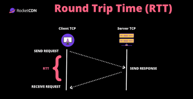
• RTT = The time taken for a small packet of data to travel across the network and return at the same point. 
• Network latency = The communication delays over a network between the server and the user. Read our complete guide about network latency and how to reduce it with a CDN .

How To Calculate Round Trip Time (RTT)

Round trip time is the average server round-trip time plus the average round trip to the final client. 

When a user requests page content on Chrome, a request is sent to the server to load that page. This request/response scheme takes time, and those “lags” are called “propagation delays”. Two propagation delays constitute one round trip time.

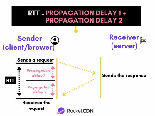
When it comes to the actual calculation, there is one simple formula to remember.

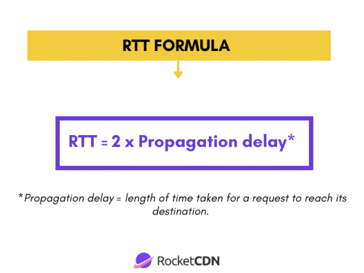
How to Fix an RTT Average

If you want to fix an RTT average, you should aim at improving the propagation delay time on both the browser and server sides. 

To calculate the total RTT average, it’s crucial to know your client’s average server RTT and Average Client RTT. 

Let’s break down the process into two simple steps.

Step 1: the calculation needs to be done on the server and client sides: 

• Average Server RTT = (RTTs1 + RTTs2)/2  
• Average Client RTT = (RTTc1 + RTTc2)/2

Step 2: then you have all the data to calculate the average total RTT

Average Total RTT = avRTTs + avRTTc

What’s a Good Round Trip Time?

A good round trip time (RTT) should be below 100 milliseconds for optimal performance. Anything above may affect the connection depending on the application. 

Example of a Round Trip Time at Microsoft 

Microsoft has guidelines and rules to maintain healthy network quality. They published their network Performance requirements from a Skype for Business client to Microsoft network Edge. Here are the performance target requirements for optimal Skype for Business media quality.

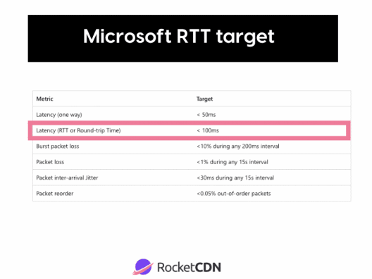
How to Check My Round Trip Time – Example

Round trip time can be seen thanks to a “ping” via the terminal command of your computer. Follow the steps below to launch the command line: 

• Open your “Terminal Command” (on Mac) or your “CMD terminal” (on Windows)
• Type “traceroute” and “yourdomain” (it also works with your IP address)
• Press “Enter”

The round-trip times (RTTs) are expressed in ms from the third to the fifth column:

How Does Round Trip Time Work?

Round trip time is based on two main parameters:

• It determines the speed at which a network can operate as well as its global reliability.
• It allows users and operators to identify how long a signal will take to complete data transmission.

What Affects Round Trip Time?

The common factors affecting Round trip time are traffic, physical distance from the user to the servers, the transmission medium, and the overall infrastructure components.

Let’s go over each factor that impacts RTT the most:

• Physical distance – the high distance between the user computer (starting point) and the server (ending point) can be responsible for a high RTT. The data transfer time will take longer if the server is located on the opposite side of the world. 
• Response time of the origin server – measured with the Time to First Byte (TTFB) metric, it’s the amount of time it takes a server to process and respond to a request. If a server is attacked with thousands of simultaneous requests (e.g, during a DDoS attack), its ability to respond efficiently will be compromised, resulting in a high RTT.
• Transmission medium – Connections are made via cables, satellite, wireless or optical fiber. Each way affects the connection speed differently.
• Local area network (LAN) traffic – if a local area is already overloaded, it can impact the connection before it reaches the public internet. 
• Node count and congestion – the connection route may encounter some issues or congestion and may be redirected several times to intermediate nodes. The more nodes are touched, the slower the connection will result in a high RTT.

What’s the Impact of RTT on Performance and How a CDN Can Help

If the RTT is too high, time-outs and performance issues are very likely to occur. The Core Web Vitals of your website will also be impacted, resulting in a poor user experience. 

Let’s take the example of the Largest Contentful Paint (LCP), which measures when the page starts loading the largest text block or image rendered on the screen. To ensure that the resource starts downloading as soon as possible, you should reduce the distance from the browser to the server. 

This is exactly the purpose of a CDN: making the content available closer to visitors.

Let’s have a closer look at the four main reasons why a CDN can help reduce the RTT and improve performance:

• CDNs decrease RTT because the users’ requests are handled by a local PoP and not the origin server, reducing the physical distance between a server and a user. CDN pops shorten the distance and improve the availability of assets, leading to an enhanced RTT.

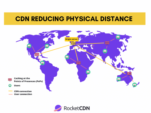
• A CDN reduces data transfer time between the cache servers and the user’s device by using caching to improve page load times. The idea is to get faster page loads for users located far away from the servers. 
• CDN helps to reduce server response time and the TTFB Time to First Byte (TTFB) metric. TTFB is the amount of time it takes for the server to get a response ready and the best way to reduce TTFB is by using a CDN to cache content. Kinsta run a performance audit before and after using a CDN, and they saw two interesting results: a faster loading site and less waiting time (TTFB).

Scenario #1 – Performance results – No CDN 

• Loading time = 1,45 s
• TTFB (wait time) = 136 ms

Scenario #2 – Performance results – With a CDN 

• Loading time = 788 ms
• TTFB (wait time) = 36 ms

• Lastly, CDNs protect your origin server in case of DDoS attacks. If your website targets an attack, a CDN will help to ensure it doesn’t reach the origin server and render your site completely offline. Thanks to the CDN, the traffic will simply be redirected to other PoPs servers, and this will help maintain a good RTT.

Using RocketCDN to Reduce RTT 

RocketCDN is a powerful CDN that uses caching and more than 35 Points of Presence to distribute the data around the globe, ensuring your website a low RTT.  It’s also very simple and easy to use – RocketCDN does all the advanced settings for you. 

Sounds promising? 

Let’s go over the best features of RocketCDN that will help boost your performance and keep your RTT below 100 ms. 

✅  RocketCDN: maintain a low RTT and TTFB but a high uptime 

Present in more than 35 markets and on four continents, RocketCDN is a powerful CDN that helps reduce RTT and TTFB. The CDN ensures fast responsiveness for all international visitors located around the globe. Nobody wants any latency to occur, and a fast website is the key to a great user experience. 

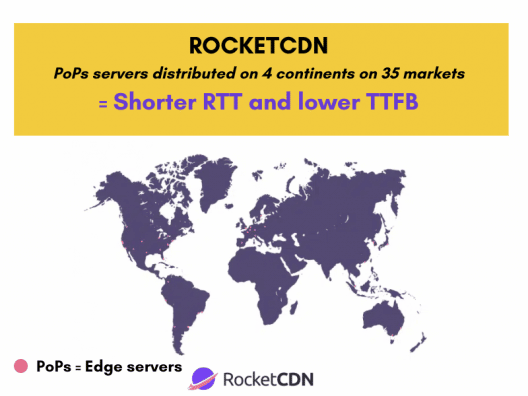
✅ Decrease the server response time with powerful caching

RocketCDN uses caching to make the content available faster for international users via PoPs, resulting in a faster server response time and increased performance. 

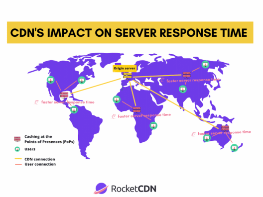
✅   Network security and DDoS attacks protection

RocketCDN includes Secure Sockets Layer (SSL) traffic and protects your origin server in case of DDoS attacks. If your website is targeted, RocketCDN will ensure that it doesn’t reach the origin server. Visitors won’t experience any downtime. They will simply be redirected to the other edge servers. And most importantly, the RTT will not be impacted!

✅ Straightforward installation and compatibility with any website technology

RocketCDN works with any website technology making it easy to connect to any CMS, including WordPress or Joomla. There is a WordPress plugin that automatically points your assets to RocketCDN.

✅  Unlimited bandwidth and high scalability 

RocketCDN can easily handle many visitors and unexpected traffic peaks with unlimited bandwidth. This is great for reducing the round trip time and avoiding any “hops” in the connection.

✅  A Cache Hit Ratio > 90% 

With a Cache Hit Ratio superior to 90%, it’s safe to say that the data is properly cached and that RocketCDN can process many requests successfully. Like RTT, Cache Hit Ratio is also an important performance metric for a CDN.    

Managing your Round trip time is straightforward with RocketCDN! 

Using RocketCDN allows you to distribute content more efficiently worldwide, save on RTT, TTFB and increase the performance of your website. RocketCDN does all the heavy lifting for you – you don’t need to worry about the technical settings! On top of that, you have up to 48 hours to cancel it if you don’t see any improvements. Try RocketCDN and start reducing your round-trip time today!

• Python Basics
• Interview Questions
• Python Quiz
• Popular Packages
• Python Projects
• Practice Python
• AI With Python
• Learn Python3
• Python Automation
• Python Web Dev
• DSA with Python
• Python OOPs
• Dictionaries

Program to calculate the Round Trip Time (RTT)

Round trip time(RTT) is the length of time it takes for a signal to be sent plus the length of time it takes for an acknowledgment of that signal to be received. This time, therefore, consists of the propagation times between the two-point of the signal. 

On the Internet, an end-user can determine the RTT to and from an IP(Internet Protocol) address by pinging that address. The result depends on various factors:- 

• The data rate transfer of the source’s internet connection.
• The nature of transmission medium.
• The physical distance between source and destination.
• The number of nodes between source and destination.
• The amount of traffic on the LAN(Local Area Network) to which end-user is connected.
• The number of other requests being handled by intermediate nodes and the remote server.
• The speed with which the intermediate node and the remote server function.
• The presence of Interference in the circuit.

Examples:  

Output: 

Please Login to comment...

Similar reads.

• Computer Networks

Improve your Coding Skills with Practice

What kind of Experience do you want to share?

• Skip to main content
• Skip to search
• Skip to select language
• Sign up for free

Round Trip Time (RTT)

Round Trip Time (RTT) is the length time it takes for a data packet to be sent to a destination plus the time it takes for an acknowledgment of that packet to be received back at the origin. The RTT between a network and server can be determined by using the ping command.

This will output something like:

In the above example, the average round trip time is shown on the final line as 26.8ms.

• Time to First Byte (TTFB)